Exercice 3 - A Deep Observation of a Globular Cluster
Globular star clusters (GC’s) usually contain about  stars.
The stars are spherically distributed, and the central densities are
about ten times larger than in open clusters. The globular clusters
are among the oldest stars in the Milky Way, and are therefore of
great importance for studies of stellar evolution. Very small
heavy element abundances, down to about
stars.
The stars are spherically distributed, and the central densities are
about ten times larger than in open clusters. The globular clusters
are among the oldest stars in the Milky Way, and are therefore of
great importance for studies of stellar evolution. Very small
heavy element abundances, down to about  times the solar value, have
been detected in some halo globular clusters. They therefore give
important information about the production of elements in the early
Universe and during the formation of the Milky Way. There are about
150-200 globular clusters in the Milky Way.
times the solar value, have
been detected in some halo globular clusters. They therefore give
important information about the production of elements in the early
Universe and during the formation of the Milky Way. There are about
150-200 globular clusters in the Milky Way.
Hertzsprung-Russell (HR) diagrams, or color-magnitude diagrams, of star clusters can be constructed in a self-consistent way without knowledge of the exact distances to them. Since the dimensions of a typical cluster are small relative to its distance from Earth, little error is introduced by assuming that each member of the cluster has the same distance modulus. As a result, plotting the apparent magnitude, rather than the absolute magnitude only amounts to shifting the position of each star in the diagram vertically by the same amount. By matching the observational main sequence of the cluster to a main sequence calibrated in absolute magnitude, the distance modulus of the cluster can be determined, giving the cluster’s distance from the observer. This method of distance determination is known as main-sequence fitting.
Rather than attempting to determine the effective temperatures of every member of a cluster by undertaking a detailed spectral line analysis of each star, it is much faster to determine their color indices (B-V). With knowledge of the apparent magnitude and the color index of each star, a colour-magnitude diagram (CMD) can be constructed.
 and
and  CCD images of the metal-poor
Galactic GC M15 (= NGC 7078) have been obtained from the ESO FORS2
imager attached to one of the four Very Large Telescope (VLT) units. The images have already
been reduced (i.e. bias substracted and flat-fielded). Analysing an HR diagram includes the following aspects:
CCD images of the metal-poor
Galactic GC M15 (= NGC 7078) have been obtained from the ESO FORS2
imager attached to one of the four Very Large Telescope (VLT) units. The images have already
been reduced (i.e. bias substracted and flat-fielded). Analysing an HR diagram includes the following aspects:
3.1 - Aperture photometry
Aperture photometry (measure the observed flux) is the most straightforward way to compute magnitudes in uncrowded or moderately crowded stellar fields. The instrumental magnitude m of a star is computed as follows:
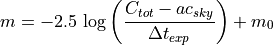
where  is the total count (star + sky) in the photometry
aperture;
is the total count (star + sky) in the photometry
aperture;  is area of the aperture in pixels squared and is roughly
equal to
is area of the aperture in pixels squared and is roughly
equal to  where
where  is the radius of the photometry aperture
in pixels;
is the radius of the photometry aperture
in pixels;  is the estimated sky value in counts per pixel
squared computed in a sky annulus centered on the star;
is the estimated sky value in counts per pixel
squared computed in a sky annulus centered on the star;  is exposure time and
  is zero point offset for the
magnitude scale.
is zero point offset for the
magnitude scale.
In practice the aperture photometry is carried out using the SExtractor software. It has also been installed on lesta, so you can execute module spider sextractor/2.19.5 to see how to load it. This software is able to provide a catalogue of objects that it identifies in the case of a single input file or it cross-matches in the case of double input files, with information that we require it to keep. An introduction to this software will be given in class. Some useful documents are also provided on our online LASTRO documentation.
Determine the optimal aperture diameter in pixels for images located in the
imagesdirectory with the single-file mode ofsextractor. This aperture represents the radius of a circle centered on the object for measuring the photons encompassed within it. The optimal value should include most of the flux from the centre object but exclude other nearby objects.- Extract the photometric information for aligned pairs of B-band and V-band images.
Use
ds9to find the aligned images, i.e., those have the glubular cluster at the same place. You will have a set of images with longer exposures and that with shorter exposures.Use
sextractorto measure the photons of stars in one band, and cross-match the object in this band to another band. Remember that the unit of the photometric information is in counts.
3.2 - Calibration or transforming to the standard system
The measurement done in the previous section is the instrumental magnitude. Conversion from instrumental magnitudes  to the calibrated magnitudes
  follows a simple linear model:


The constants to account for the instrumental effect  and
and  can be determined using “standard stars”, which are stars with determined magnitudes and colours, observed with the same instrument and filters and under identical conditions as the M15 cluster. Don’t forget to have a look to headers of fits files as well!
For the atmospheric extinction coefficients  and
and  , one can use the average atmospheric absorption coefficients measured at Paranal :
  [mag / airmass], and
  [mag / airmass].
  is the airmass (
 where
where  is the altitude of the star measured from zenith).
For simplicity, in this exercise we will ignore second-order colour coefficients  and
and  , which are negligible compared to other terms. They can be determined using “standard stars” as well.
Interstellar reddening and extinction are due to the presence of dust grains along the line-of-sight. While the former affects the measured colour, the latter affects the observed luminosity. We consider a reddening correction of 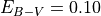 . As interstellar exctinction has generally the same origin as the reddening, the exctinction correction can be approximated by the relation
 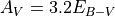 .
.
Measure
and for standard stars with the calibrated magnitude provided in Ru152.pdfunder thestandard_stardirectory.Obtain the apparent magnitude in B- and V-band with corrections in instrument, atmospheric extinction, interstellar reddening and extinction
Now you should have two CMD at hand, one with longer exposure and the other with shorter exposure.
3.3 - Fiducial sequence and isochrones
Compare the CMDs with the fiducial sequence, choose the one that contains more information. Describe the morphology of that CMD, i.e. link the different regions of the diagram with the phases of stellar evolution and locate the main-sequence turn-off point (TO), i.e. the point where the stars are currently leaving the main-sequence. The so-called “fiducial sequence” is a smoothed sequence of M15 obtained by e.g. P.R. Durrell and W.E. Harris (1993, AJ 105, 1420), which just represents some kind of best fit to the observed sequence (
evolution_models/fiducial.txt).- In this exercise, you need isochrones corresponding to the metallicity of M15, namely
![[\rm{Fe/H}]=-2.15](../../_images/math/581ef2c0c408569c332313300d281a45b495aae4.png) , which corresponds to a fraction of “heavy” elements
, which corresponds to a fraction of “heavy” elements 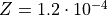 , and its Helium composition of 0.2. Isochrones refer to curves connecting stars in CMD with the same composition and age, but various masses. Such isochrones were computed by Vandenberg (1985, ApJS 58, 561) for similar metallicities. See the file
 ReadMe.txtfor a detailed description of filesevolution_models/*85iso.txt. Determine the distance of M15 by compare your CMD with a calibrated zero-age main-sequence (ZAMS).
Estimate the age of M15 by fitting isochrones to the CMD fiducial sequence.
- In this exercise, you need isochrones corresponding to the metallicity of M15, namely
Estimate the half-light radius of M15.
Estimate the luminosity and mass of M15 assuming the cluster consists in solar-type stars only.