Exercice 5 - Introduction to Cosmological N-body Simulations¶

(This exercise is inspired from a hands-on session given by Volker Springel in 2013)

In this practical work, we will simulate the evolution of a portion of a $\Lambda\mathrm{CDM}$ universe, from very high redshift up to the present time. The work is divided into the following steps:

5.0 - Setup lesta

5.1 - Generate the initial conditions

5.2 - Run the simulation

5.3 - Analyse the results

As a complement to this page, you can read this presentation (pdf file).

You will need to have a personal directory in the /scratch directory on lesta. Ask the system manager (by emailing astro-it-support@unige.ch) in order to get one. You will also need special privileges to run jobs using sbatch, so ask for this as well at the same time.

5.0 - Setup lesta¶

Make sure you are familiar with the lesta documentation before starting this exercise. (Note: avoid using a conda environment while compiling the C code. Run conda deactivate before loading the modules.)

We will be using openmpi version 1.10.2 due to compatibility reasons with the C codes involved. Load this by typing

$ module add GCC/4.9.3-2.25
$ module add OpenMPI/1.10.2
$ module add FFTW/2.1.5

5.1 - Generate the initial conditions¶

Initial conditions for cosmological simulations are based on the power spectrum of visible matter in our large-scale Universe. The latter is derived from direct observations provided by large galaxy surveys, weak lensing surveys, Lyman alpha absorption, and also from the cosmic microwave background.

To generate initial conditions for cosmological simulations, we usually proceed through the following steps :

Setup a Cartesian grid with dimensions corresponding to the volume of the simulated universe. Periodic boundaries will be applied.

Compute the perturbation field using the inverse Fourier transform of the power spectrum.

Compute the perturbation of the velocities following the Zel’dovich approximation.

Apply these perturbations to the Cartesian grid.

Different codes have been developed to generate initial conditions. Here, we will use a parallel code called N-GenIC developed by Volker Springel. In order to use this code, you need to :

Download it. You can do this, for example, inside a directory called TP4 that you create in your home directory. To be able to download files from URLs, you need to be connected to one of the login nodes (e.g. login01, login02, etc.) rather than on lesta (which is used to perform the actual computations).
$ mkdir TP4
$ cd TP4

$ wget http://www.mpa-garching.mpg.de/gadget/n-genic.tar.gz
$ tar -xzf n-genic.tar.gz
$ cd N-GenIC/
Edit the Makefile by adding the following lines above the first instance of “ifeq ($(SYSTYPE), …)”
ifeq ($(SYSTYPE),"lastro_TP4")
CC = mpicc
OPTIMIZE = -Wall
GSL_INCL =
GSL_LIBS =
FFTW_INCL= -I /opt/ebsofts/MPI/GCC/4.9.3-2.25/OpenMPI/1.10.2/FFTW/3.3.4/include
FFTW_LIBS= -L /opt/ebsofts/MPI/GCC/4.9.3-2.25/OpenMPI/1.10.2/FFTW/3.3.4/lib
MPICHLIB =
endif
which sets the paths to some required libraries. In order to use these definitions when we compile the code, change the line
SYSTYPE="OPA-Cluster64-Gnu"
to
SYSTYPE="lastro_TP4"
Note that there will be many “SYSTYPE=…” lines that are commented out (i.e. ignored by the compiler) above the one you change.
Back at the command line, compile the code.
$ make
If successful, this will create a binary called N-GenIC in the current directory. (Don’t worry if you get a few warnings about unused variables.)

In order to execute N-GenIC, we need to provide it with some parameters. An example file containing these parameters is given in “ics.param”. Useful parameters are:

parameter name	value	description
`Box`	150000.0	Periodic box size of simulation
`Omega`	0.3	Total matter density (at z=0)
`OmegaLambda`	0.7	Cosmological constant (at z=0)
`HubbleParam`	0.7	Hubble parameter
`Sigma8`	0.9	Power spectrum normalization
`Redshift`	63	Starting redshift

You can leave these as their default values.

HubbleParam corresponds to the commonly used little $h$ , which is linked to the Hubble constant through:

$H_0 = 100\cdot h \frac{\mathrm{km}}{\mathrm{s}\cdot\mathrm{Mpc}} = 3.2407789\,10^{-18}\, h\, s^{-1}$

Units are defined by the following parameters

parameter name	value	description
`UnitLength_in_cm`	3.085678e21	defines length unit of output (in cm/h)
`UnitMass_in_g`	1.989e43	defines mass unit of output (in g/h)
`UnitVelocity_in_cm_per_s`	1e5	defines velocity unit of output (in cm/s)

For the sake of simplicity, change the parameter controlling the number of files written in parallel to 1, i.e.

NumFilesWrittenInParallel 1

Other parameters may be kept unchanged. To run the code, simply type

$ mkdir ICs
$ ./N-GenIC ics.param

You should end up with a file called ICs/ics.

5.2 - Run the simulation¶

In the previous part, we have setup initial conditions, where positions, velocities, and masses of $N$ particles have been defined. The second step is to let the system evolve under gravitational forces. We will hereafter neglect all other types of forces, for example pressure forces. We thus assume that the system is composed of collisionless dark matter only.

Basically, what we need to do is to integrate $N$ equations of motion, where $N$ corresponds to the number of particles. At each time step, the forces acting on each particle depend on the positions of all others. On top of that, the expansion of the universe must be taken into account. By using a so-called ‘comoving’ reference frame, it is possible to absorb the expansion of the universe into the equations of motion.

In practice, computing the forces on $N$ particles due to $N-1$ other particles is far from trivial, as the problem scales as $N^2$ . We will simply use here an open source code called Gadget-2 designed to solve this kind of problem. The full documentation for Gadget-2 may be found here.

In order to use Gadget-2, do the following:

From your working directory (e.g. ~/TP4), download and extract the Gadget-2 source code.
$ wget http://www.mpa-garching.mpg.de/gadget/gadget-2.0.7.tar.gz
$ tar -xzf gadget-2.0.7.tar.gz
$ cd Gadget-2.0.7/Gadget2/
Edit the Makefile with the following changes :
increase the size of the mesh needed by the particle mesh (PM) gravity solver
OPT   +=  -DPMGRID=256
This will better suit our $128^3$ particle set-up.
do not use the hdf5 format (comment out the line)
#OPT   +=  -DHAVE_HDF5
compute the potential energy
OPT   +=  -DCOMPUTE_POTENTIAL_ENERGY
write the potential and acceleration in the snapshot files
OPT   +=  -DOUTPUTPOTENTIAL
OPT   +=  -DOUTPUTACCELERATION
as previously, add a block that defines the path to some needed libraries
ifeq ($(SYSTYPE),"lastro_TP4")
CC = mpicc
OPTIMIZE = -O3 -Wall
GSL_INCL =
GSL_LIBS =
FFTW_INCL= -I /opt/ebsofts/MPI/GCC/4.9.3-2.25/OpenMPI/1.10.2/FFTW/3.3.4/include
FFTW_LIBS= -L /opt/ebsofts/MPI/GCC/4.9.3-2.25/OpenMPI/1.10.2/FFTW/3.3.4/lib
MPICHLIB =
endif
In order to use this block, change
SYSTYPE="MPA"
to
SYSTYPE="lastro_TP4"
Compile.
$ make
This should compile the code and create a binary called Gadget2.

Now, prepare the directory where you will run the simulation.

Then, assuming that your user name is lastro_etu, create a directory that will contain the simulation.
$ mkdir /scratch/lastro_etu/lcdm256-001
$ cd /scratch/lastro_etu/lcdm256-001
Copy the sources into this directory that you just compiled.
$ rsync -av ~/TP4/Gadget-2.0.7/Gadget2/ src
(This assumes you have downloaded gadget into a folder called TP4 in your home directory. Change the path to suit your setup if necessary.)
Similarly copy the initial conditions.
$ rsync -av ~/TP4/N-GenIC/ICs .
Create a new directory that will store the output files.
$ mkdir snap
Create a file that will contain the list of time coordinates (as scale factors) of when you want to store snapshots. (A snapshot refers to the state of the entire system at a fixed moment in time.)
$ ./gmktimesteps.py -p 5 > outputs.txt
Before doing so, you need to copy gmktimesteps.py to your folder
$ cp /home/astro/jacevedo/TP-IV-utilities/some-Gtools/gmktimesteps .
Copy an example parameter file.
$ rsync -av ~/TP4/Gadget-2.0.7/Gadget2/parameterfiles/lcdm_gas.param params
Edit this file to setup specific parameters for your configuration:
InitCondFile               ICs/ics
OutputDir                  snap/
[...]
OutputListFilename         outputs.txt
Set the beginning and end of the simulation to scale factors corresponding to a redshift of 63 and 0 (present day):
TimeBegin                  give a value here
TimeMax                    give a value here
Verify the cosmological parameters, as well as the size of the box. These must be the same as the ones used in N-GenIC:
Omega0                0.3
OmegaLambda           0.7
OmegaBaryon           0.0
HubbleParam           0.7
BoxSize               150000.0
Set a gravitational softening length of order $\sim 1/35$ the mean particle spacing, fixed in comoving coordinates:
SofteningHalo             give a value here
[...]
SofteningHaloMaxPhys      give a value here
(It might help to recall that our simulation has $128^3$ particles.)

And finally, run the simulation. As we will run it in parallel using the queue system of lesta (see the documentation), you first need to create a batch script, which we’ll call “start.slurm”. In this file, put

#!/bin/bash
#SBATCH

srun --mpi=pmi2 src/Gadget2 params

Then, to submit the job, simply type

$ sbatch -p p4 -J mysim -n 8 start.slurm

This will run the simulation on the queue named p4 using 8 cpus.

To check that your simulation is running, type

$ squeue

and you should see your job listed. Using 8 cpus, the simulation should take less than one hour. Output files will be generated in the snap directory. The file slurm-xxxxxx.out contains the standard I/O outputs. You can tail it to follow the progress of the simulation:

$ tail -n 100 slurm-xxxxxx.out

5.3 - Analyse the results¶

Let’s take a look at it¶

It is always interesting to have a look at a simulation, as the human eye is very good at spotting suspicious artefacts. Using some tools provided with the python pNbody package. The modules that contained pNbody were lost during the transition from Lesta01 to Lesta02-04. We can access them again using:

$  module use /home/astro/revazy/local/soft/modulefiles/
$  module add clastro/yggdrasil

You first need to set the proper formats file for pNbody. Do this by adding a (hidden) configuration folder to your home directory:

$ mkdir -p ~/.pNbody/formats

In formats/, put this file called gadget.py (also included in the data resources).

Now, in the directory of the simulation, create a directory called film, and move into it. There, create a file called filmparam.py, with the following content:

#global film

film = {}
film['ftype']  = "gadget"
film['time']   = "nb.atime"
film['exec']   = "nb.translate([-nb.boxsize/2.,-nb.boxsize/2.,-nb.boxsize/2.])"

film['format'] = 'png'
film['frames'] = []

frame = {}
frame['width']      = 512
frame['height']     = 512
frame['size']       = (160000/2.,160000/2.)
frame['tdir']       = None
frame['pfile']      = None
frame['exec']       = None
frame['macro']      = None
frame['components'] = []

component = {}
component['id']        = '#all'
component['rendering'] = 'map'

# append component to frame
frame['components'].append(component)

# append frame to film
film['frames'].append(frame)

The movie is then created using the python executable gmkgmov applied on all of the snapshots created from your simulation:

$ gmkgmov -p filmparam.py --imdir pngs ../snap/snapshot_0*

This should generate a set of images, one from each snapshot, in a new directory called pngs.

You can now encode the movie as a typical ‘.avi’ file and view it. To do this, we need to load modules that conflict with the previously loaded modules (because they use different versions of GCC). The easiest way to solve this is to exit lesta (or the node you are working on) and login back again. Also, visualizing the movie requires that you connect to lesta with the -Y parameter (X forwarding): ssh -Y username@login01.astro.unige.ch. You can access an interactive node by running:

$ srun -p p5 --pty $SHELL

Once inside a fresh node, load the necessary modules and generate the movie:

$ module load GCC/11.2.0
$ module load OpenMPI/4.1.1
$ module load FFmpeg/4.3.2
$ module load MPlayer/1.5

# encode
$ ffmpeg -y -i pngs/%04d_0000-#all-000000.png -vcodec mpeg4 -b:v 50000k film-x264.avi
# watch
$ mplayer film-x264.avi

If the simulation was successful, you should see the growth of large scale structures. At $z=0\, (a=1)$ the universe should be similar to the one displayed in Fig. 2.

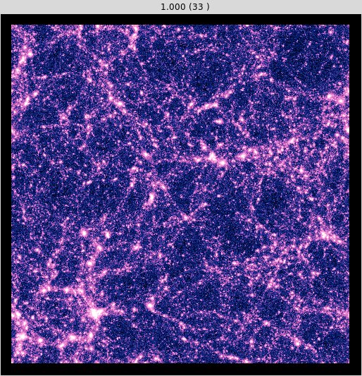
../../_images/lcdm.jpg — **Fig.2** : Surface density of a simulated universe at $z=0 (a=1)$ .¶

Extracting haloes¶

In the previous section, we have seen that from the initially nearly homogeneous universe, structures emerge and grow under the action of gravity. At $z=0$ , a large number of clusters (or haloes) seem to be present. In order to characterise the state of the universe at $z=0$ , it is common to compute the so-called “halo mass function”, i.e., the number of haloes within a given range of mass.

However, to do so, it is first necessary to extract those haloes from the final snapshot. This part is far from trivial and different algorithms exist for this purpose. In this work, we will use the classical Friends of Friends (FoF) algorithm, implemented here in a code called FoF_Special kindly provided by Volker Springel.

In short, the idea of a FoF algorithm is the following: each particle belongs to a group of particles made of neighbouring particles (friends) lying within a distance smaller than a given linking length (a fixed parameter). If two particles have one or more common neighbouring particles, the group is merged. At the end of the procedure, a number of groups exist. The algorithm guarantees that within a group, all particles are friends of friends of friends etc. and that no particles outside of this group have friends inside of the group. That is, no particle in the group is situated at a distance smaller than the linking length with respect to any particle outside.

To use FoF_Special first download it and extract it in the same directory where you extracted gadget-2.0.7.tar.gz and n-genic.tar.gz:

$ wget http://lastro.epfl.ch/misc/TP4/doc/_downloads/fof.tar.gz
$ tar -xzf fof.tar.gz
$ cd FoF_Special/

Before compiling, we need to setup the linking length. This is hardcoded in the file main.c, and its value is given in term of mean particle separation. You can leave its default value.

double LinkLength = 0.2;

Then, compile the code by typing

$ make

If you encounter an error related to stddef.h, it means the wrong C compiler is being used. Edit the Makefile so that the compiler specification line reads

CC      = gcc

Try compiling again by running

$ make clean
$ make

You should end up with a binary called FoF_Special. To apply FoF_Special on the snapshots of our simulation we will proceed as follows:

In the directory where you ran the simulation, create a folder called fof and copy FoF_Special that you just created.
Then, run FoF_Special on the last snapshot, which should correspond to $z=0$ . You need to provide FoF_Special with three arguments: the output directory, the basename of the snapshot files, and the number of the output for which you want to extract haloes. This yields:
```
./FoF_Special . ../snap/snapshot 32
```
Three directories are created: groups_catalogue, groups_indexlist, groups_particles. Each contains a file labeled with the snapshot number. Files in the directory groups_catalogue contain information on the groups, while groups_particles contains the positions of particles in groups. We will not use the files in the directory groups_indexlist.

In order to use the output files, we provide students with a small python library that will help the reading of these files. The module is given in the FoFlib.py script. Note that you will likely need to modify the lines in the methods where files are opened to read:

f = open(filename,'rb')

since the files to be read are in binary format.

The mass function of dark haloes¶

One common way to characterise the structure of a universe is to measure the statistical properties of its haloes. The simplest statistic we can perform is to count the number of haloes found for a given mass interval, normalised to the volume of the universe that contains those structures. This function is usually called the “halo mass function”.

The structure of dark haloes¶

According to the $\Lambda\mathrm{CDM}$ paradigm, galaxies form inside dark haloes. Studying the structures of those haloes allows us to make a direct link between the predictions of numerical simulations and observations. Thus, once haloes have been extracted, it is interesting to compute properties like their density profiles or rotation curves.

Exercices

Write a code that enables you to extract and center the top 10 most massive haloes.

HINT: Instead of using simply the center of mass (as provided by FoFlib.py), you need to compute the center of the system as the minimum of the gravitational potential of the halo. Recall that the potential at position $\boldsymbol{x}$ for a system of particles is given by

$\Phi(\boldsymbol{x}) = -\sum_i^N \frac{G m_i}{|\boldsymbol{x} - \boldsymbol{x}_i|},$

where $m_i$ and $\boldsymbol{x}_i$ are the mass and position of particle $i$ .
For each extracted halo, compute the values of $r_{200}$ and $M_{200}$ . These quantities are sometimes called the virial radius and the virial mass, respectively. The latter is defined as the mass enclosed within a sphere of mean density equal to 200 times the critical density of the universe ( $\rho_{\mathrm{c}}$ ):

$\frac{M_{200}}{(4\pi/3) r_{200}^3} = 200\,\rho_{\mathrm{c}}$
Plot the mass density profiles of these haloes (i.e. spherically averaged density as a function of radius), normalised to the critical density of the universe, between the softening length and the virial radius.

BONUS: Try to see if you can fit each measured radial density function with a Navarro-Frenk-White (NFW) profile.

BONUS: Determine which halo in your catalogue best corresponds to the Milky Way by considering the (average) circular velocity as a function of radius.