Display Models

Generate the example file

To run the examples of this section, you must first move to the ~/pnbody_examples directory. If the latter does not exists, you can first create it with:

pNbody_copy-examples

then inside this directory, type:

./scripts/mkmodel_for_display.py

This will create the N-body file snapd.dat. This file contains a rotating disk of radius 30, with a small plummer sphere centered on (15,15,10).

The display method

Any model may be displayed simply using the method NbodyDefault.display(). This method takes several parameters that will be described in detail below. For our first example, we simply use the size parameter, which set the size of the displayed area:

>>> from pNbody import *
>>> nb = Nbody("snapd.dat",ftype='gadget')
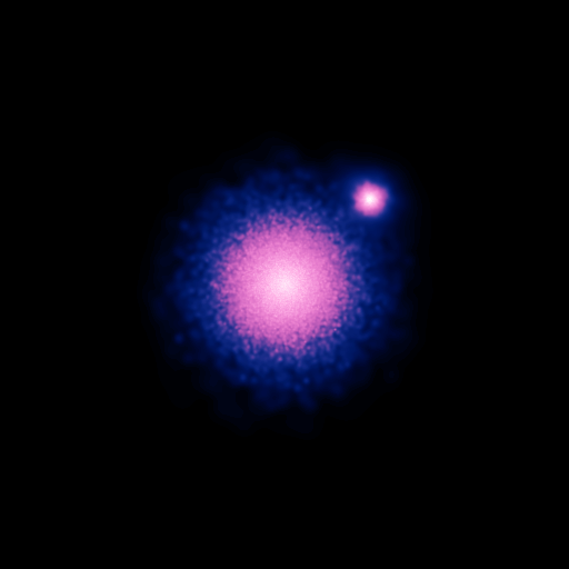
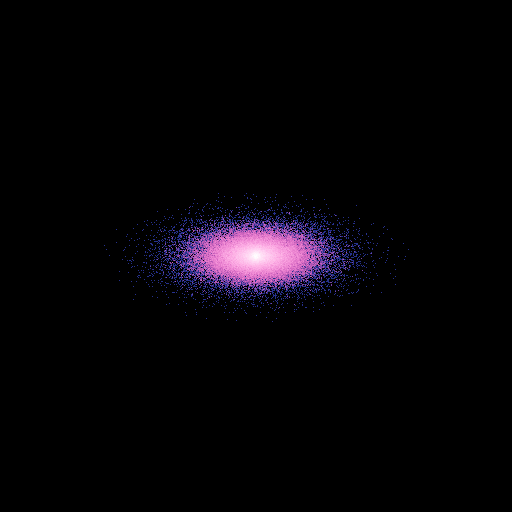
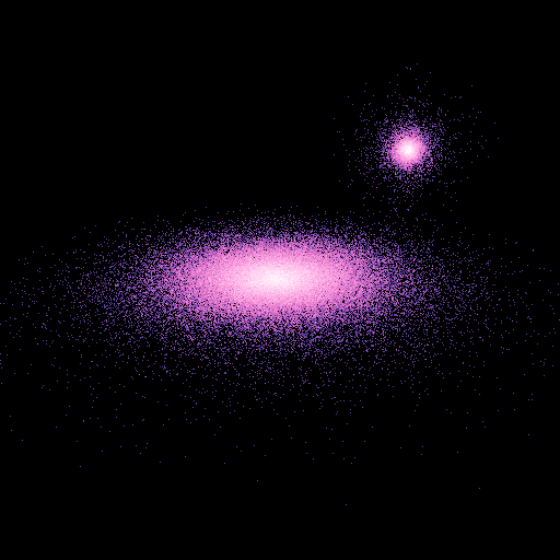
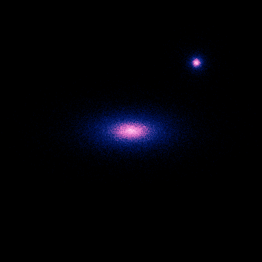
>>> nb.display(size=(50,50))

If your default parameters are still the ones of the pNbody distribution, this should display the following image:

Display parameters

pNbody provides rather complex tools to display N-body systems. The tools uses different parameters that are sumarized in the following table:

name	meaning	value	type
obs	observer	None	(ArrayObs)
xp	observing position	None	(List)
x0	position of observer	None	(List)
alpha	angle of the head	None	(Float)
view	view	xz	(String)
r_obs	dist. to the observer	201732.223771	(Float)
clip	clip planes	(100866.11188556443, 403464.44754225772)	(Tuple)
cut	cut clip planes	no	(String)
eye	name of the eye	None	(String)
dist_eye	distance between eyes	-0.0005	(Float)
foc	focal	300.0	(Float)
persp	perspective	off	(String)
shape	shape of the image	(512, 512)	(Tuple)
size	pysical size	(6000, 6000)	(Tuple)
frsp	frsp	0.0	(Float)
space	space	pos	(String)
mode	mode	m	(String)
rendering	rendering mode	map	(String)
filter_name	name of the filter	None	(String)
filter_opts	filter options	[10, 10, 2, 2]	(List)
scale	scale	log	(String)
cd	cd	0.0	(Float)
mn	mn	0.0	(Float)
mx	mx	0.0	(Float)
l_n	number of levels	15	(Int)
l_min	min level	0.0	(Float)
l_max	max level	0.0	(Float)
l_kx	l_kx	10	(Int)
l_ky	l_ky	10	(Int)
l_color	level color	0	(Int)
l_crush	crush background	no	(String)
b_weight	box line weight	0	(Int)
b_xopts	x axis options	None	(Tuple)
b_yopts	y axis options	None	(Tuple)
b_color	line color	255	(Int)

The value of these parameters may be obtained by the command:

pNbody_show-parameters

Set the observer position

When creating an image from a model, one has to choose the observer position, the look at point and the orientation of the head. The user has tree possibilities to define these parameters :

1. Define manually the observer matrix obs. obs is a 4x3 array matrix. Meaning of the four vectors composing this matrix is given in the following table :

obs	Meaning
obs[0]	position of the observer
obs[1]	position of the look at point (with respect to the position of the observer)
obs[2]	position of the head (with respect to the position of the observer)
obs[3]	position of the arm (with respect to the position of the observer)

If obs is defined, it is used in priority.

2. Using the parameters xp, x0 and alpha, where x0 is the observer position, xp is the look at point and alpha the angle between the head and the z axis.

3. Using the parameters view and r_obs. This simpler method is used if obs, xp and x0 are set to None. The parameter view can be equal to xy, xz or yz, the projection being parallel to one of the main axis. r_obs gives the distance between the observer and the look at point.

Example:

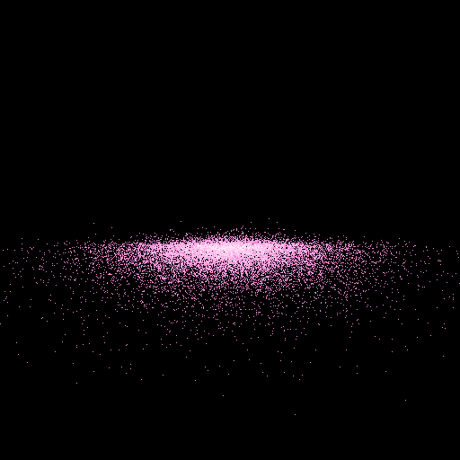
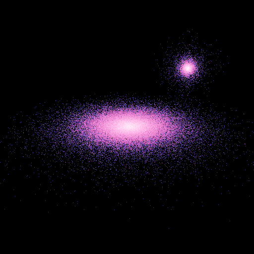
To see the disk face-on, projecting it along the z axis:

>>> nb.display(obs=None,x0=None,xp=None,size=(50,50),view='xy')

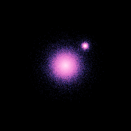
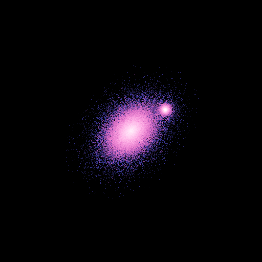
To align the center of the disk with the center of the sphere:

>>> nb.display(obs=None,x0=[30.,30.,20.],xp=[15,15,10],alpha=0,size=(50,50))

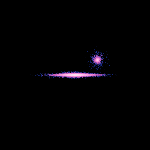
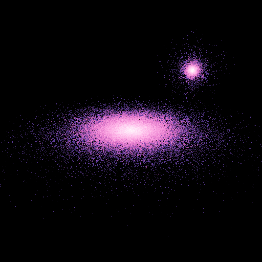
To look at the disk from the bottom, tilting the head from 45 degres:

>>> nb.display(obs=None,x0=[0,-50,-50],xp=[0,0,0],alpha=pi/4,size=(50,50))

Set the projection mode

pNbody offers two projection modes. If persp``='on', the model is projectec using a frustrum projection matrix. In the other case, it uses an ortho matrix (orthogonal projection). The near and far clipping planes are given by the parameter ``clip containing a tuple. The left, right, bottom and top clipping planes are given by the parameter size. If cut is set to ‘yes’, particles outside the box defined by the 6 planes are not displayed.

Example:

Using the frustrum projection:

>>> nb.display(obs=None,x0=[0,-50,20],xp=[0,0,0],alpha=0,size=(5,5),persp='on',clip=(10,50))

The field of view is determined using clip and size.

If cut is set to yes, only particles inside the clip planes are displayed:

>>> nb.display(obs=None,x0=[0,-50,20],xp=[0,0,0],alpha=0,size=(5,5),persp='on',clip=(10,50),cut='yes')

Stero mode

In order to create stereo images, you can specify the eye you are looking with (‘right’,’left’). When exposition the model using the method NbodyDefault.expose(), the observer will be rotate around an axis parallel to its head, with a center rotation in the direction of the look at point, at a distance foc of the eye. The angle of the rotation is such as to move the observer of a distance dist_eye/2.

Example:

Left and right images may be obtained respectively with:

>>> nb.display(obs=None,x0=[0,-50,20],xp=[0,0,0],alpha=0,size=(5,5),persp='on',clip=(10,50),foc=100,dist_eye=0.01,eye='left')
>>> nb.display(obs=None,x0=[0,-50,20],xp=[0,0,0],alpha=0,size=(5,5),persp='on',clip=(10,50),foc=100,dist_eye=0.01,eye='right')

This gives the following image that may be seen using a cross-eyed vision:

Shape of the final image

The shape in pixel of the final image is set by the tuple shape.

Display space

The space parameter may be either pos (default) or vel. In the second case, the model is displayed in velocity space, this simply means that the positions are replaced by the velocities.

Example:

The model in the velocity space gives:

>>> nb.display(obs=None,x0=None,size=(1,1),view='xy',space='vel')

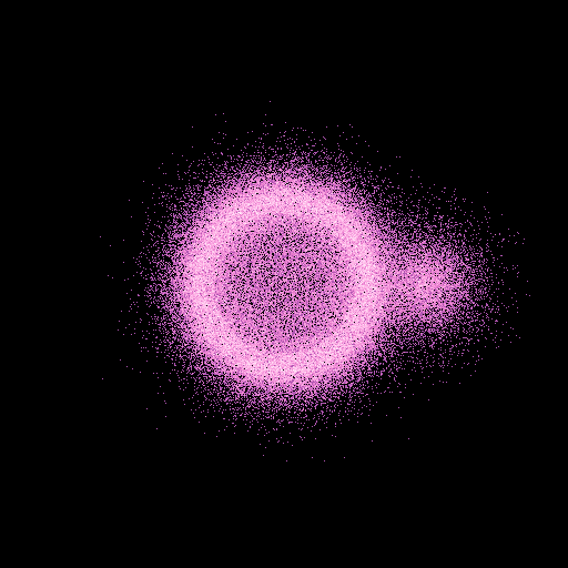
We clearly see the ofset of (0.5,0,0) in velocity of the sphere.

Display mode

The mode parameter is very important. It tells the method NbodyDefault.display() which physical quantities must be displayed. By default, it value is m, meaning the mass. When used, a projected mass map (surface density) is returned.

The value of mode parameter may be set to:

1. a value from the following list. In this case, the value does not dependends on the observer position :

Value	Meaning	Formula
“m”	zero momentum	\(\sum m\)
“x”	first momentum in x
“y”	first momentum in y
“z”	first momentum in z
“x2”	second momentum in x
“y2”	second momentum in y
“z2”	second momentum in z
“vx”	first velocity momentum in x	\(\sum m vx\)
“vy”	first velocity momentum in y	\(\sum m vy\)
“vz”	first velocity momentum in z	\(\sum m vz\)
“vx2”	second velocity momentum in x	\(\sum m vx^2\)
“vy2”	second velocity momentum in y	\(\sum m vy^2\)
“vz2”	second velocity momentum in z	\(\sum m vz^2\)
“lx”	first specific kinetic momemtum in x
“ly”	first specific kinetic momemtum in y
“lz”	first specific kinetic momemtum in z
“Lx”	first kinetic momemtum in x
“Ly”	first kinetic momemtum in y
“Lz”	first kinetic momemtum in z
“u”	first momentum of specific energy
“rho”	first momentum of density
“T”	first momentum of temperature
“A”	first momentum of entropy
“P”	first momentum of pressure
“Tcool”	first momentum of cooling time
“Lum”	first momentum of luminosity
“Ne”	first momentum of electronic density

2. a value from the following list. In this case, the value does dependends on the observer position :

Value	Meaning	Formula
“r”	first momentum of radial distance
“r2”	second momentum of radial distance
“vr”	first momentum of radial velocity
“vr2”	second momemtum of radial velocity
“vxyr”	first momentum of radial velocity in the plane	\(\sum m (x vx + y vy)/\sqrt{x^2+y^2}\)
“vxyr2”	second momentum of radial velocity in the plane	\(\sum m [(x vx + y vy)/\sqrt{x^2+y^2}]^2\)
“vtr”	first momentum of tangential velocity in the plane	\(\sum m (x vx - y vy)/\sqrt{x^2+y^2}\)
“vtr2”	second momentum of tangential velocity in the plane	\(\sum m [(x vx - y vy)/\sqrt{x^2+y^2}]^2\)

3. any scalar linked with each particle, for example the density nb.rho.

Example:

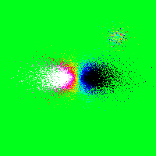
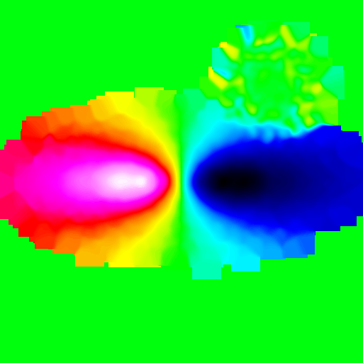
A radial velocity map is obtained using mode=vr:

>>> nb.display(obs=None,x0=[0,-50,25],xp=[0,0,0],alpha=0,size=(30,30),mode='vr',scale='lin',palette='rainbow4')

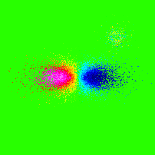
Note that we have used a linear scale here.

Rendering

The parameter rendering is by default set to map. This means that particles are projected on a grid (2d histrogram). However, in some circumstances, it may be usefull to display simple objects, like a cube or a sphere, determined by a small number of points. The object is obtained by linking all points with segments. This is done by setting the parameter rendering to one of the following value:

Value	Call	Meaning
lines	draw_lines	draw a continuous line linking all points
segments	draw_segments	draw disconnected segemnts (need persp=’on’)
points	draw_points	draw individual points
polygon	draw_polygon	draw a continuous closed line
polygon2	draw_polygonN 2	draw polygons with groups of 2 points
polygon4	draw_polygonN 4	draw polygons with groups of 4 points
polygon10	draw_polygonN 10	draw polygons with groups of 10 points
polygon#	draw_polygonN n	draw polygons with groups of n points

Examples:

>>> from pNbody import ic
>>> nb = ic.box(20,1,1,1)
>>> nb.display(shape=(256,256),size=(1.1,1.1))

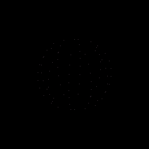
>>> nb.display(shape=(256,256),size=(1.1,1.1),rendering='points')

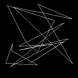
>>> nb.display(shape=(256,256),size=(1.1,1.1),rendering='lines')

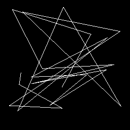
>>> nb.display(shape=(256,256),size=(1.1,1.1),rendering='polygon')

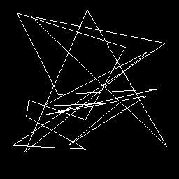
>>> nb.display(shape=(256,256),size=(1.1,1.1),rendering='segments',persp='on')

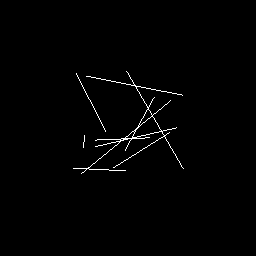
>>> nb.display(shape=(256,256),size=(1.1,1.1),rendering='polygon4')

Lets now display the sphere.dat model

>>> from pNbody import *
>>> nb = Nbody("sphere.dat",ftype='gadget')
>>> nb.display(obs=None,x0=[-50,-50,25],xp=[0,0,0],alpha=0,size=(2,2))

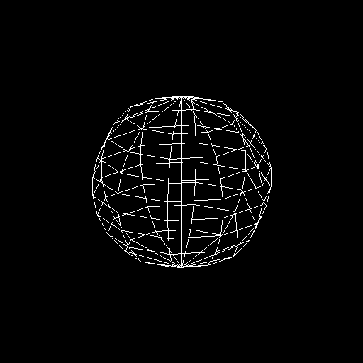
This model is a discretised sphere. using rendering='polygon' this gives:

>>> nb.display(obs=None,x0=[-50,-50,25],xp=[0,0,0],alpha=0,size=(2,2),rendering='polygon')

Set color range

Once a mapping has been performed, it return a matrix containing physical values. The latter must be transformed into an image coded by 256 colors, i.e, a matrix containing integers between 0 and 255. The transformation from the initial matrix and the integer matrix is determined using four parameters:

Parameter	Meaning
scale	the scaling ‘lin’ or ‘log’
cd	if scale=’lin’, this gives the position of the elbow
mn	the minimum physical value
mx	the maximum physical value

In more details, if \(M_p\) is the physical matrix and \(M_i\) the integer one, the transformation is:

1. when scale = ‘lin’:

\[M_i = 255 \frac{M_p-mn}{mx-mn}\]

2. when scale = ‘log’:

\[M_i = 255 \left( \frac{\log( 1+\frac{M_p-mn}{cd}) }{ \log(1+ \frac{mx-mn}{cd}) } \right)\]

If mn = 0 or mx = 0, or cd = 0, these parameters are set automatically.

Examples:

To cut the velocities at a values of -0.3 and 0.3 in the velocity map example:

>>> nb.display(obs=None,x0=[0,-50,25],xp=[0,0,0],alpha=0,size=(30,30),mode='vr',scale='lin',mn=-0.2,mx=0.2,palette='rainbow4')

To change the contrast of an image:

>>> nb.display(obs=None,x0=[0,-50,25],xp=[0,0,0],alpha=0,size=(30,30),cd=1e2)

Set filters

Its possible to apply filter on the physical matrix, before converting it into an integer matrix. To set a filter, you must specify the filter_name parameter and the filter_options parameter: The actual filters are :

Filter name	filter opts
convol	[nx,ny,sx,xy]
convolve	[nx,ny,sx,xy]
boxcar	[nx,ny,sx,xy]
gaussian	[sigma]
uniform	[sigma]

Examples:

>>> nb.display(obs=None,x0=[0,-50,25],xp=[0,0,0],alpha=0,size=(30,30),mode='vr',scale='lin',palette='rainbow4',filter_name='gaussian',filter_opts=[5])

Draw contours

It is possible to add contours

Parameter	Meaning
l_n	number of levels
l_min	mininum level value
l_max	maximum level value
l_kx	smoothing size in x
l_ky	smoothing size in x
l_color	color code
l_crush	‘yes’ or ‘no’ , if yes, display only contours

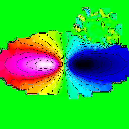
Examples:

>>> parameters = {}
>>> parameters['obs'] = None
>>> parameters['x0'] = [0,-50,25]
>>> parameters['xp'] = [0,0,0]
>>> parameters['alpha'] = 0
>>> parameters['size'] = (30,30)
>>> parameters['mode'] = 'vr'
>>> parameters['scale'] = 'lin'
>>> parameters['palette'] = 'rainbow4'
>>> parameters['filter_name'] = 'gaussian'
>>> parameters['filter_opts'] = [5]
>>> parameters['l_n'] = 20
>>> parameters['l_min'] = -0.2
>>> parameters['l_max'] = -0.2
>>> parameters['l_color'] = 255
>>> nb.display(parameters,palette='rainbow4')

Draw axis

It is possible to draw a very simple axis around an image, using the following parameters:

Parameter	Meaning
b_weight	weight of the line
b_xopts	x ticks options (m0,d0,h0,m1,d1,h1) m=dist between ticks, d=first tick h=height of the ticks
b_yopts	y ticks options (m0,d0,h0,m1,d1,h1) m=dist between ticks, d=first tick h=height of the ticks
b_color	smoothing size in x

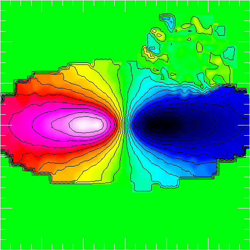
Examples:

>>> parameters['b_weight'] = 1
>>> parameters['b_xopts'] = 1
>>> parameters['b_xopts'] = None
>>> parameters['b_yopts'] = None
>>> parameters['b_color'] = 255
>>> nb.display(parameters,palette='rainbow4')

frsp

This last parameter is used to smooth the image using an adaptative smoothing length. Typically, in N-body system, the adaptative smoothing length may be the one derived using the SPH technique. When the particles are projected in the focal plane, each particle is convolved whith a kernel corresponding to its proper smoothing length multiplied by the parameter frsp. This allows to play with the strength of the smooting. The value of the smoothin length must be stored in th variable nb.rsp..

Examples:

Here, we first use the NbodyDefault.ComputeSph() method to compute the SPH radius of each particle. This radius is determined a the radius of a sphere containing 50 neighbors with a maximal deviation of 1. As this method automatically store the results to nb.Hsml we have to copy it to nb.rsp, before calling the display function:

>>> nb.ComputeSph(DesNumNgb=50,MaxNumNgbDeviation=1)
>>> nb.rsp = nb.Hsml
>>> nb.display(obs=None,x0=None,xp=None,size=(50,50),view='xy',frsp=2)