Using pNbody with the python interpreter
In order to use this tutorial, you first need to follow the steps given in the the section Generate examples . Assuming you are in the example directory, you can simply follow the instructions below.
First, start the python interpreter:
leo@obsrevaz:~/pNbody_examples python3
Python 2.4.2 (#2, Jul 13 2006, 15:26:48)
[GCC 4.0.1 (4.0.1-5mdk for Mandriva Linux release 2006.0)] on linux2
Type "help", "copyright", "credits" or "license" for more information.
>>>
Now, you can load the pNbody module as well as the numpy one:
>>> from pNbody import Nbody
>>> import numpy as np
Creating pNbody objects from scratch
We can first start by creating a default pNbody objet and get info about it
>>> nb = Nbody()
>>> nb.info()
-----------------------------------
particle file       : ['file.dat']
ftype               : 'default'
mxntpe              : 6
nbody               : 0
nbody_tot           : 0
npart               : [0, 0, 0, 0, 0, 0]
npart_tot           : [0, 0, 0, 0, 0, 0]
mass_tot            : 0.0
byteorder           : 'little'
pio                 : 'no'
>>>
All variables linked to the object nb are accesible by typing nb. followed by the associated variables :
>>> nb.nbody
0
>>> nb.mass_tot
0.0
>>> nb.pio
'no'
Now, you can create an object by giving the positions of particles:
>>> pos = np.ones((10,3),np.float32)
>>> nb = Nbody(pos=pos)
>>> nb.info()
-----------------------------------
particle file       : ['file.dat']
ftype               : 'default'
mxntpe              : 6
nbody               : 10
nbody_tot           : 10
npart               : array([10,  0,  0,  0,  0,  0])
npart_tot           : array([10,  0,  0,  0,  0,  0])
mass_tot            : 1.00000011921
byteorder           : 'little'
pio                 : 'no'

len pos             : 10
pos[0]              : array([ 1.,  1.,  1.], dtype=float32)
pos[-1]             : array([ 1.,  1.,  1.], dtype=float32)
len vel             : 10
vel[0]              : array([ 0.,  0.,  0.], dtype=float32)
vel[-1]             : array([ 0.,  0.,  0.], dtype=float32)
len mass            : 10
mass[0]             : 0.10000000149
mass[-1]            : 0.10000000149
len num             : 10
num[0]              : 0
num[-1]             : 9
len tpe             : 10
tpe[0]              : 0
tpe[-1]             : 0
In this case, you can see that the class automatically intitialize other arrays variables (vel, mass, num and rsp) with default values. Only the first and the last element of each defined vector are displyed by the methode info. All defined arrays and array elements may be easily accessible using the numarray convensions. For exemple, to display and change the positions of the tree first particles, type:
>>> nb.pos[:3]
array([[ 1.,  1.,  1.],
       [ 1.,  1.,  1.],
       [ 1.,  1.,  1.]], type=float32)
>>> nb.pos[:3]=2*np.ones((3,3),np.float32)
>>> nb.pos[:3]
array([[ 2.,  2.,  2.],
       [ 2.,  2.,  2.],
       [ 2.,  2.,  2.]], type=float32)
Open from existing file
Now, lets try to open the gadget snapshot gadget_z00.dat. This is achieved by typing:
>>> nb = Nbody('gadget_z00.dat',ftype='gadget')
Again, informatins on this snapshot may be obtained using the instance info():
>>> nb.info()
-----------------------------------
particle file       : ['gadget_z00.dat']
ftype               : 'Nbody_gadget'
mxntpe              : 6
nbody               : 20560
nbody_tot           : 20560
npart               : array([ 9160, 10280,     0,     0,  1120,     0])
npart_tot           : array([ 9160, 10280,     0,     0,  1120,     0])
mass_tot            : 79.7066955566
byteorder           : 'little'
pio                 : 'no'

len pos             : 20560
pos[0]              : array([-1294.48828125, -2217.09765625, -9655.49609375], dtype=float32)
pos[-1]             : array([ -986.0625    , -2183.83203125,  4017.04296875], dtype=float32)
len vel             : 20560
vel[0]              : array([ -69.80491638,   60.56475067, -166.32981873], dtype=float32)
vel[-1]             : array([-140.59715271,  -66.44669342,  -37.01613235], dtype=float32)
len mass            : 20560
mass[0]             : 0.00108565215487
mass[-1]            : 0.00108565215487
len num             : 20560
num[0]              : 21488
num[-1]             : 1005192
len tpe             : 20560
tpe[0]              : 0
tpe[-1]             : 4

atime               : 1.0
redshift            : 2.22044604925e-16
flag_sfr            : 1
flag_feedback       : 1
nall                : [ 9160 10280     0     0  1120     0]
flag_cooling        : 1
num_files           : 1
boxsize             : 100000.0
omega0              : 0.3
omegalambda         : 0.7
hubbleparam         : 0.7
flag_age            : 0
flag_metals         : 0
nallhw              : [0 0 0 0 0 0]
flag_entr_ic        : 0
critical_energy_spec: 0.0

len u               : 20560
u[0]                : 6606.63037109
u[-1]               : 0.0
len rho             : 20560
rho[0]              : 7.05811936674e-11
rho[-1]             : 0.0
len rsp             : 20560
rsp[0]              : 909.027587891
rsp[-1]             : 0.0
len opt             : 20560
opt[0]              : 446292.5625
opt[-1]             : 0.0
You can obtain informations on physical values, like the center of mass or the total angular momentum vector by typing:
>>> nb.cm()
array([-1649.92651346,   609.98256428, -1689.04011033])
>>> nb.Ltot()
array([-1112078.125 ,  -755964.1875, -1536667.125 ], dtype=float32)
In order to visualise the model in position space, it is possible to generate a surface density map of it using the display instance:
>>> nb.display(size=(10000,10000),shape=(256,256),palette='light')
You can now performe some operations on the model in order to explore a specific region. First, translate the model in position space:
>>> nb.translate([3125,-4690,1720])
>>> nb.display(size=(10000,10000),shape=(256,256),palette='light')
>>> nb.display(size=(1000,1000),shape=(256,256),palette='light')
Ou can now rotate around:
>>> nb.rotate(angle=np.pi)
>>> nb.display(size=(1000,1000),shape=(256,256),palette='light')
You can now display a temperature map of the model. First, create a new object with only the gas particles:
>>> nb_gas = nb.select('gas')
>>> nb_gas.display(size=(1000,1000),shape=(256,256),palette='light')
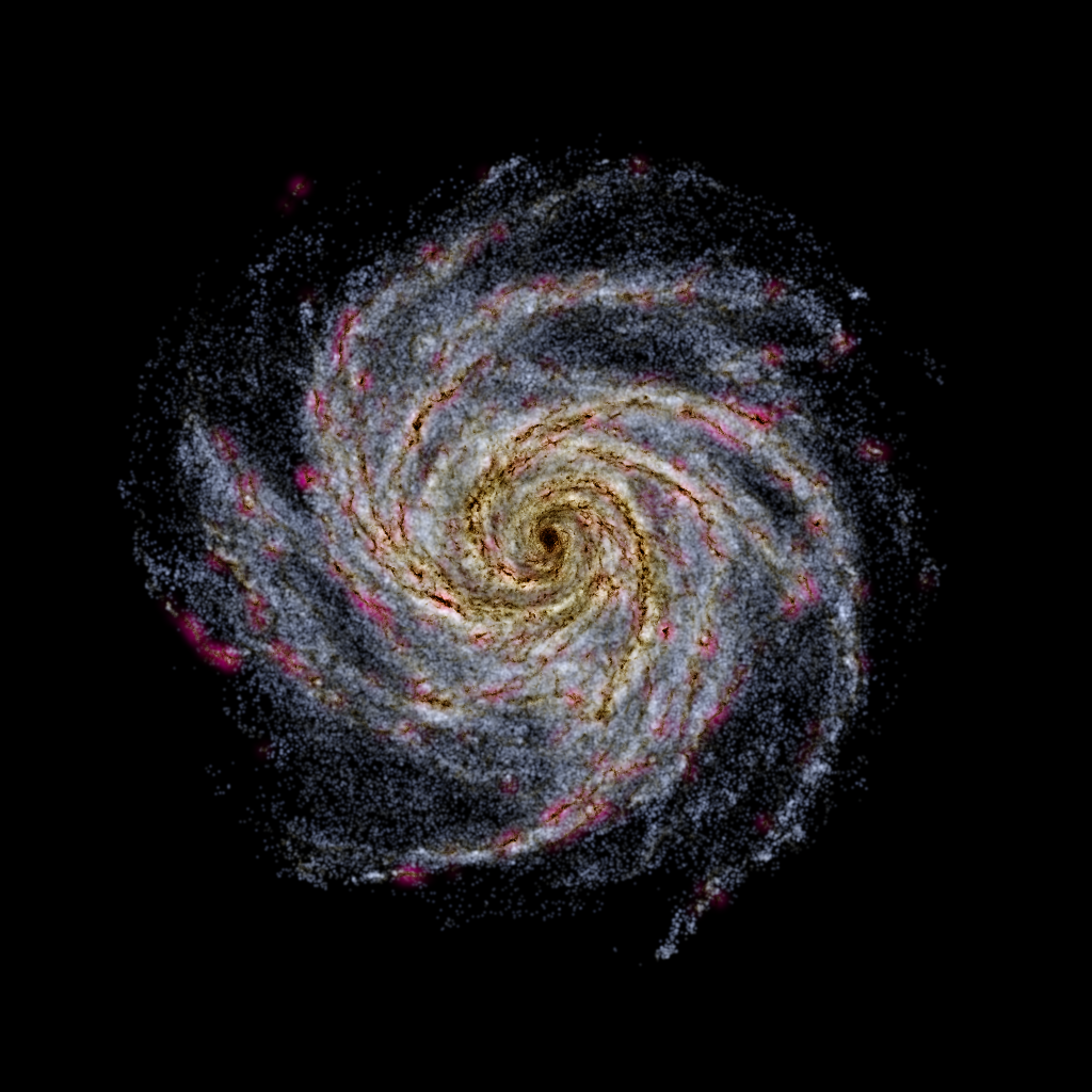
now, display the temperture mass-weighted map:
>>> nb_gas.display(size=(1000,1000),shape=(256,256),palette='rainbow4',mode='T',filter_name='gaussian')
To render the gas density, a cool feature is to convolve each particle with a kernel of size of the
sph smoothing length. This is done setting a factor frsp corresponding to the smoothing value.
Warning : a large value will requires a very large amount of time to compute:
>>> nb_gas.display(size=(5000,5000),shape=(512,512),palette='light',mode='m',scale="log",frsp=0.1)
Selection of particles
You can select only particles within a radius smaller tha 500 (in user units) with respect to the center:
>>> nb_sub = nb.selectc((nb.rxyz()<500))
>>> nb_sub.display(size=(1000,1000),shape=(256,256),palette='light')
Now, rename the new model and save it:
>>> nb_sub.rename('gadget_z00_sub.dat')
>>> nb_sub.write()
A new gadget file has been created and saved in the current directory. We can now select particles as a function of the temperature. First, display the maximum temperature among all gas particles, then selectc particles and finally save in ‘T11.num’ the identifier (variable num) of these particles:
>>> np.log10(max(nb_gas.T()))
6.8904919420046244
>>> nb_sub = nb_gas.selectc( (nb_gas.T()>1e5) )
>>> nb_sub.write_num('T11.num')
Now open a new snapshot, from the same simulation, but at different redshift and find the particles in previous snapshot with temperature higher than $10^{11}$:
>>> nb = Nbody('gadget_z40.dat',ftype='gadget')
>>> nb.display(size=(10000,10000),shape=(256,256),palette='light')
>>> nb_sub = nb.selectp(file='T11.num')
>>> nb_sub.display(size=(10000,10000),shape=(256,256),palette='light')
Now, instead of saving it in a gadget file, save it in a swift file type. You simply need to call the set_ftype instance before saving it:
>>> nb = nb.set_ftype('swift')
>>> nb.rename('swift.hdf5')
>>> nb.write()
Merging two models
As a last example, we show how two pNbody models can be easyly merged with only 11 lines:
>>> nb1 = Nbody('disk.dat',ftype='gadget')
>>> nb2 = Nbody('disk.dat',ftype='gadget')
>>> nb1.rotate(angle=np.pi/4,axis=[0,1,0])
>>> nb1.translate([-150,0,0])
>>> nb1.vel = nb1.vel + [50,0,0]
>>> nb2.rotate(angle=np.pi/4,axis=[1,0,0])
>>> nb2.translate([+150,0,50])
>>> nb2.vel = nb2.vel - [50,0,0]
>>> nb3 = nb1 + nb2
>>> nb3.rename('merge.dat')
>>> nb3.write()
Now display the result from different point of view:
>>> nb3.display(size=(300,300),shape=(256,256),palette='lut2')
>>> nb3 = nb3.select('disk')
>>> nb3.display(size=(300,300),shape=(256,256),palette='lut2',view='xz')
>>> nb3.display(size=(300,300),shape=(256,256),palette='lut2',view='xy')
>>> nb3.display(size=(300,300),shape=(256,256),palette='lut2',view='yz')
>>> nb3.display(size=(300,300),shape=(256,256),palette='lut2',xp=[-100,0,0])
or save it into a gif file:
>>> nb3.display(size=(300,300),shape=(256,256),palette='lut2',xp=[-100,0,0],save='image.gif')