Radial velocity fitting with DACE
This document describes the procedure to follow to perform a few actions with the DACE radial velocity (RV) analysis tool.
Accessing the RV analysis tool
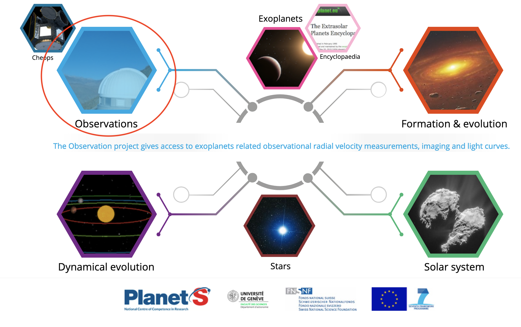
Go to the DACE homepage.
Click on "Observations".
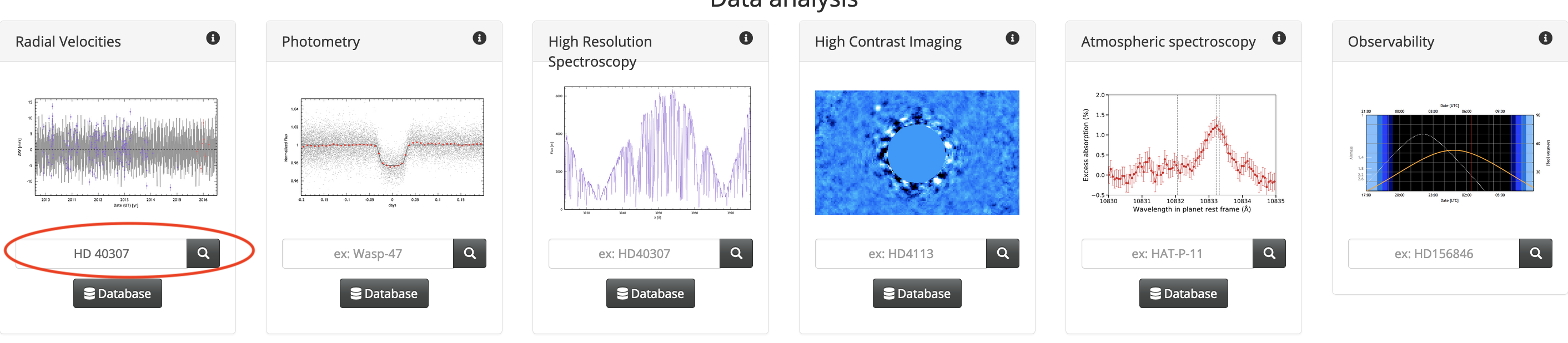
Enter the name of the system you want to analyse.
Data visualization
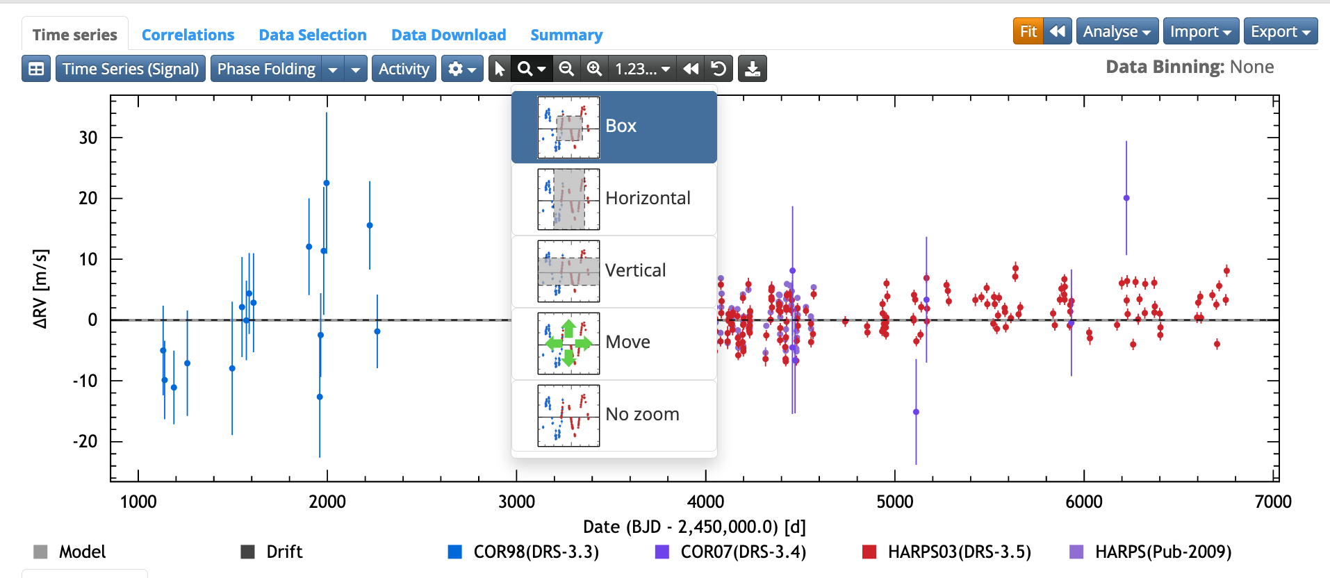
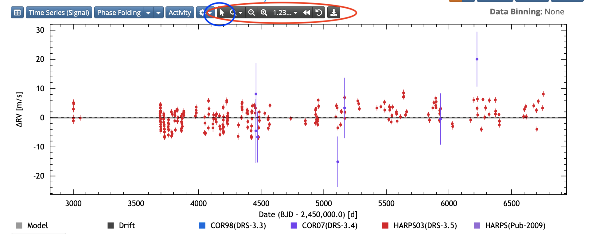
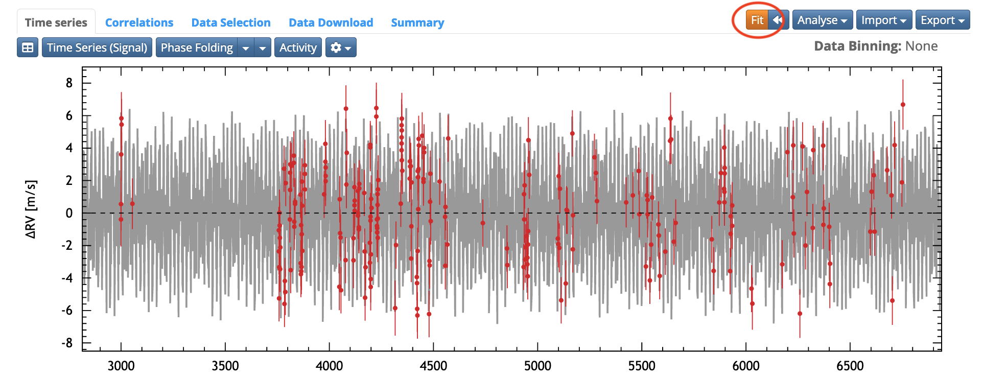
Once the data is loaded, you see a plot of the time-series.
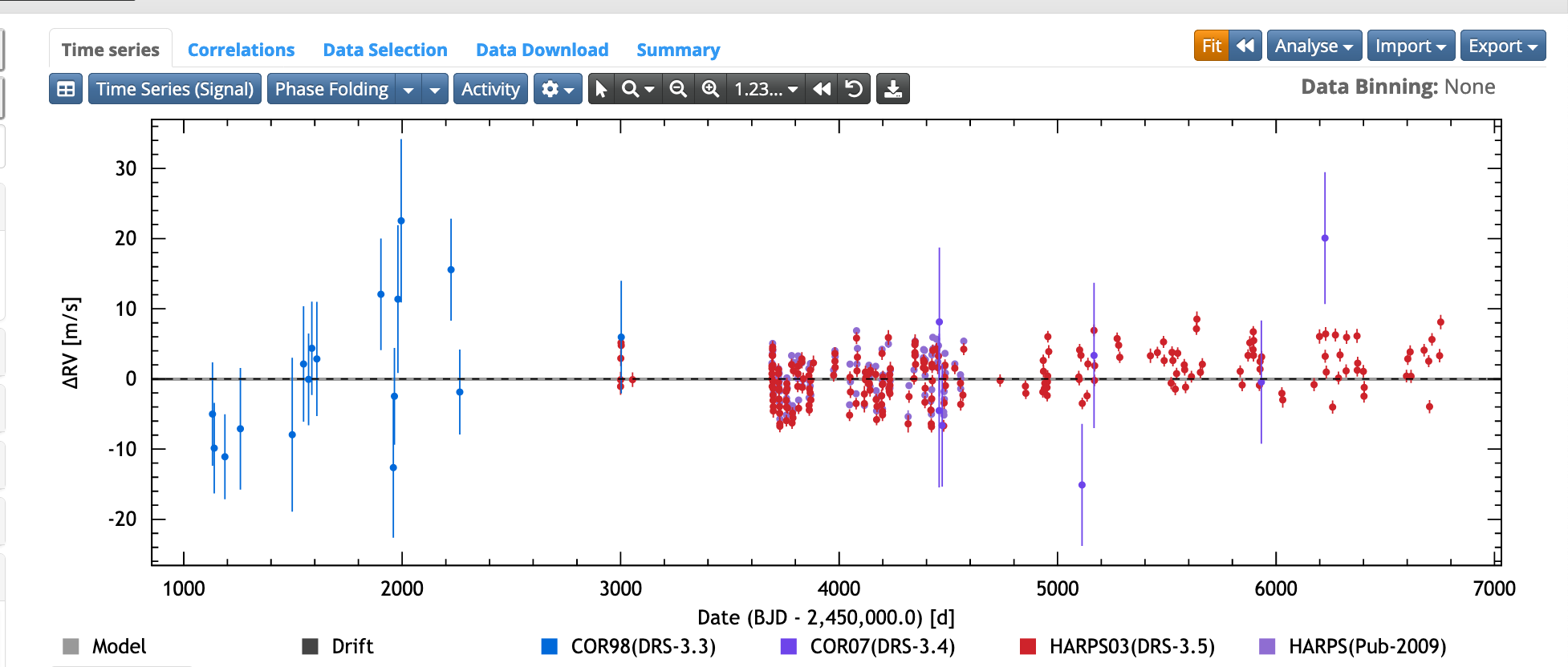
You can zoom on the time series by selecting zoom options (in red).
To go back to the original view, click on the icon within the blue circle.

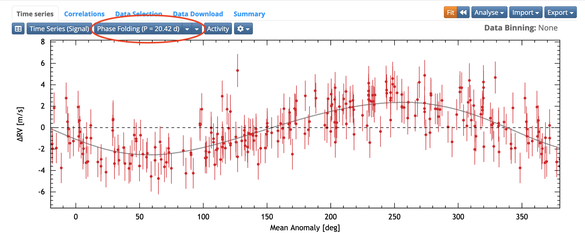
Phase-folding
Once you have added at least one planet, click on the phase-folding icon several times to see the data phase-folded on the different periods of the "Keplerian signals" section.
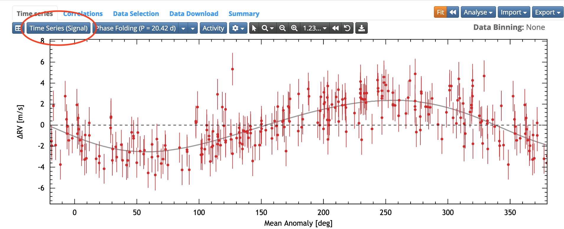
Time series
To go back to the time series view from phase-folding.
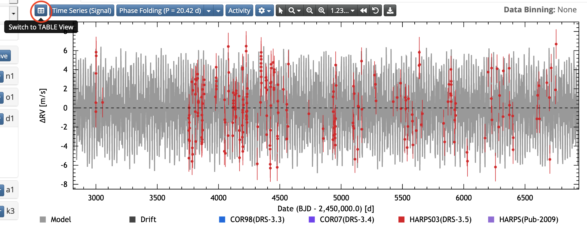
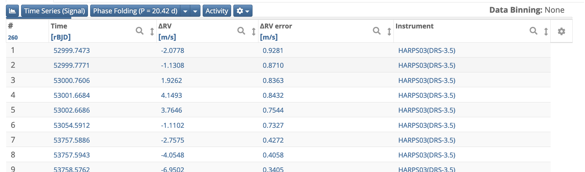
Information on the data
Switch to table view
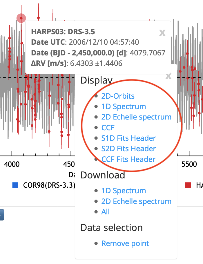
Spectra
Visualise the spectra corresponding to one data point. Click on the data point of interest and select the data product you are interested into.
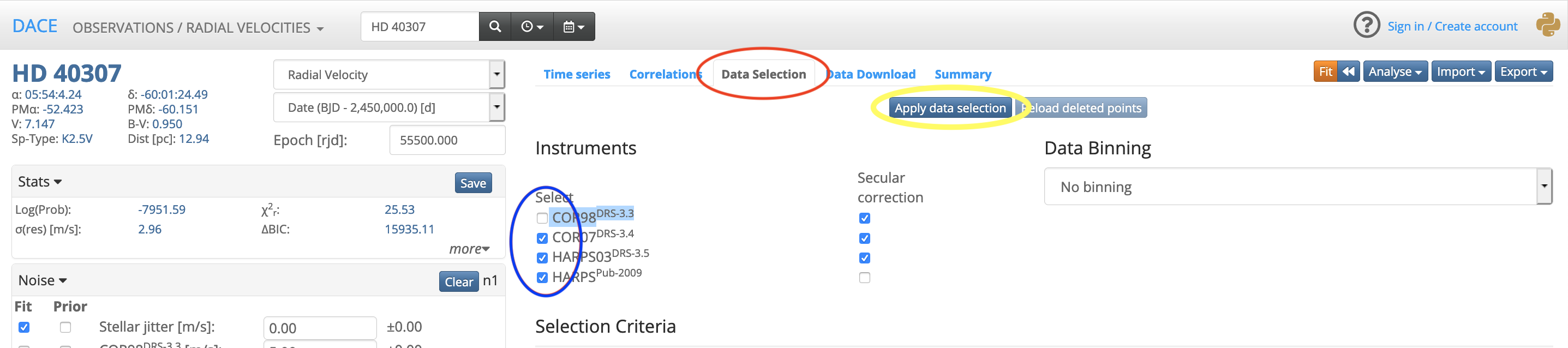
Data selection
Select instruments
1. Go to the Data selection tab (in red) 2. select or unselect instruments (blue) 3. click on "apply data selection" (yellow).
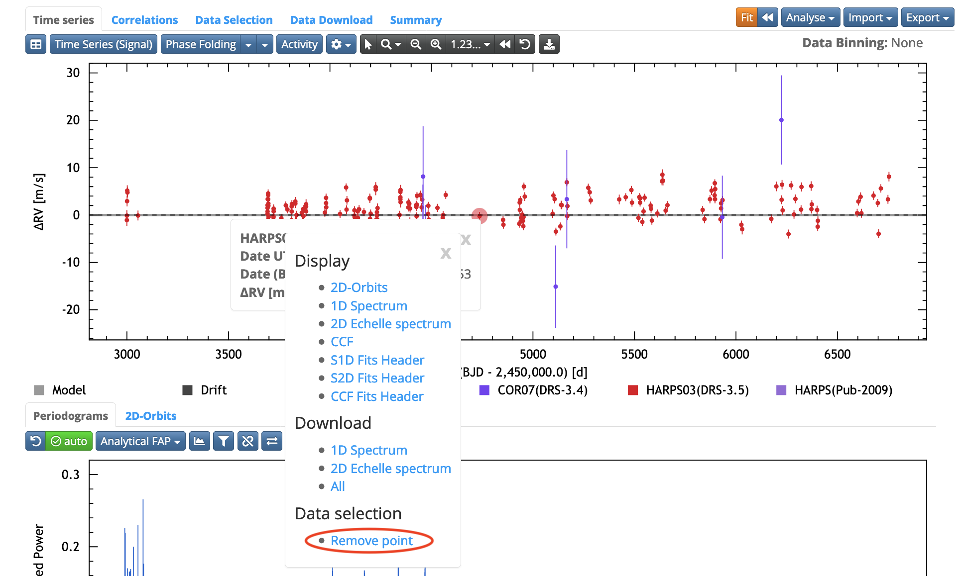
Removing one data point
Click on the data point, then on "Remove point".
Removing several points at the same time
Select the cursor (blue) within the toolbar (red).
Select the shape of the selection.
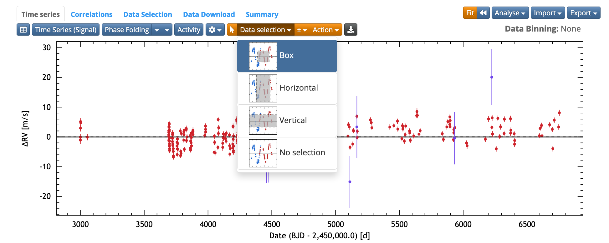
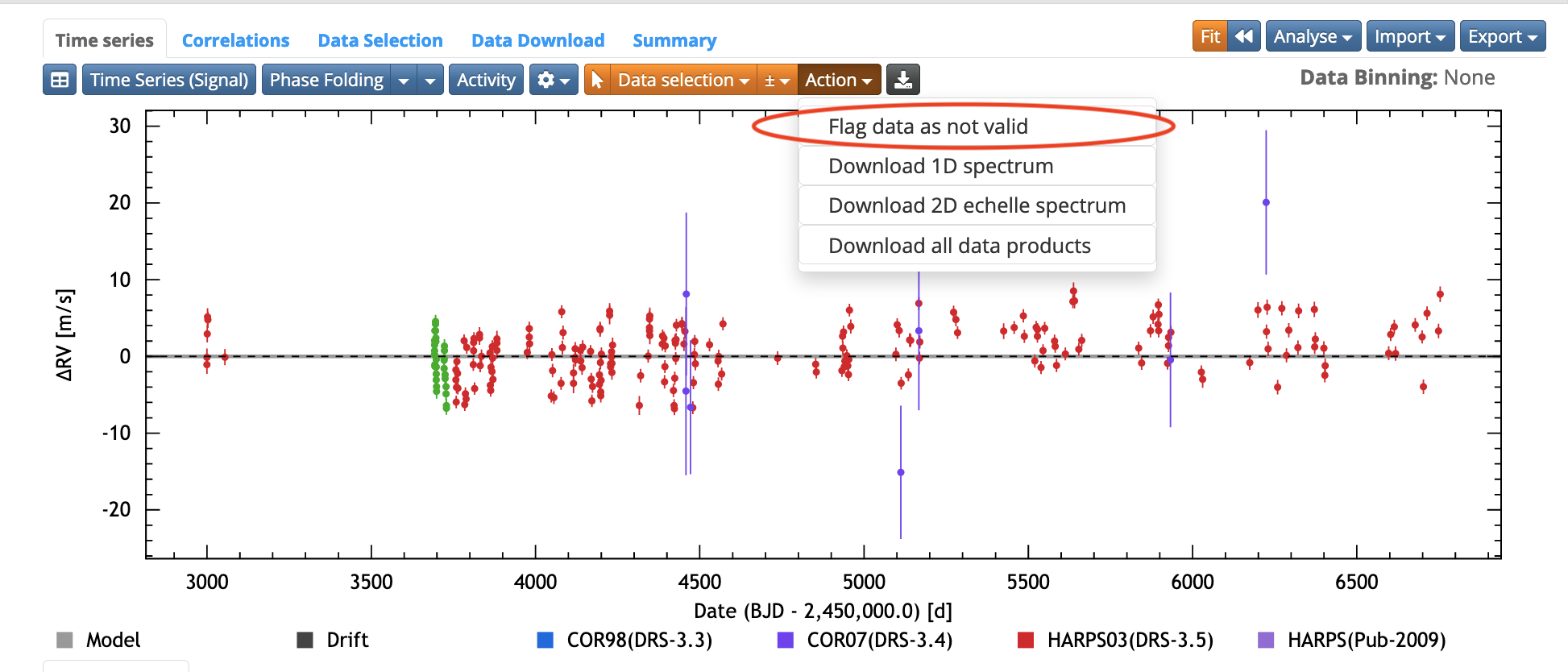
Once you have selected the points, they appear in green. Go to "actions", and select "flag data as not valid".
Reload deleted data points
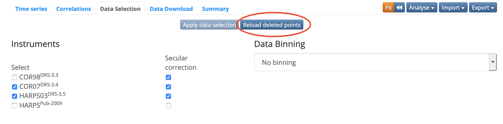
If you want to re-include data that were deleted,
go to the Data selection tab and click on "reload deleted points".
RV analysis
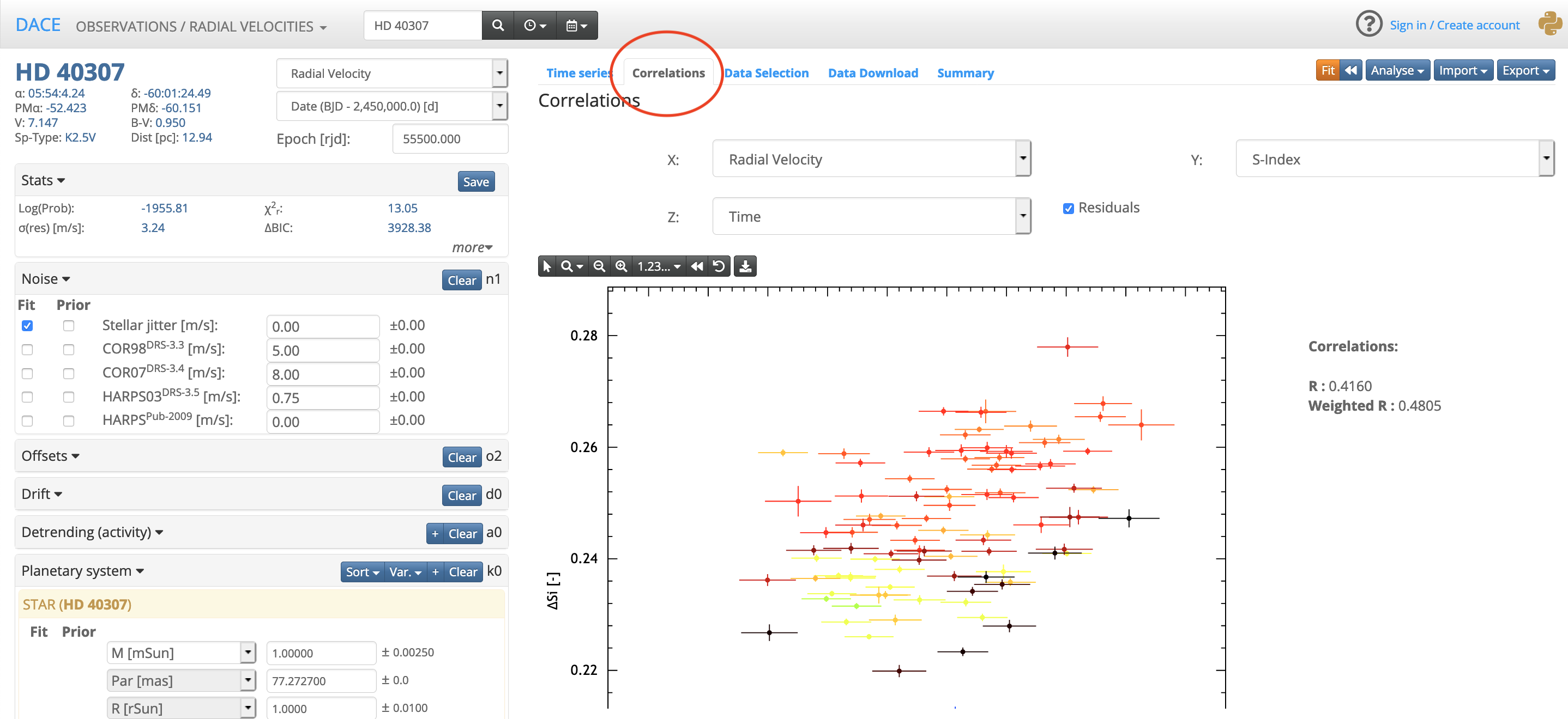
Checking correlations with ancillary indicators
Go to the Correlations tab.
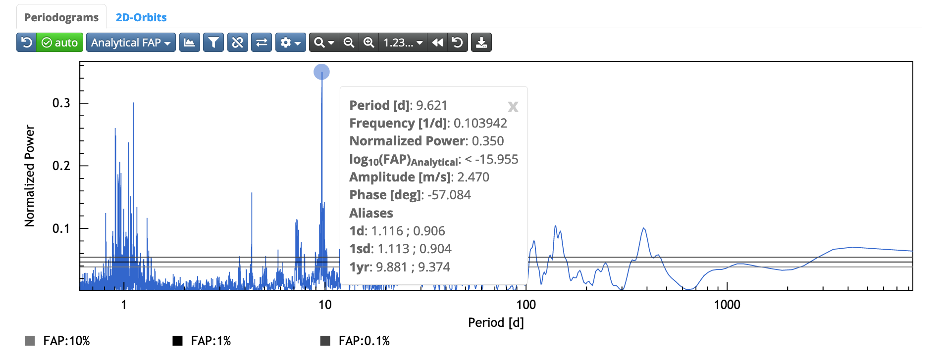
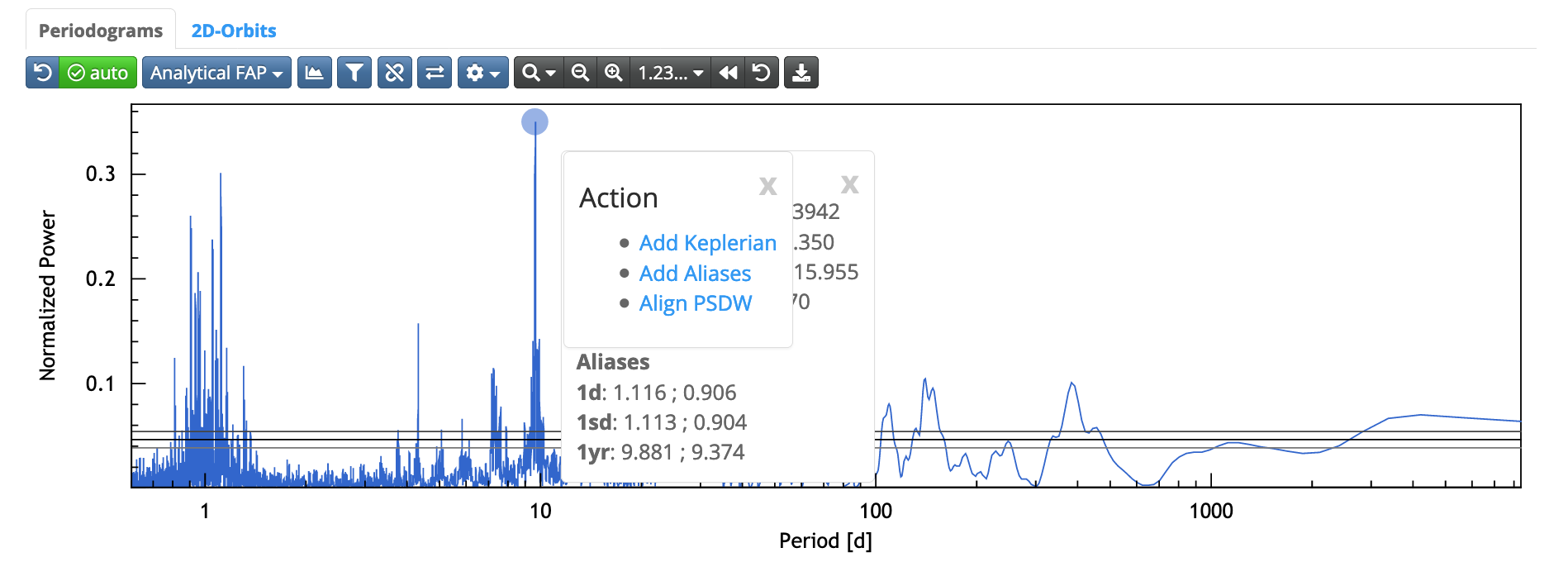
Periodogram
False alarm probability: place the cursor on the periodogram to see the false alarm probability of the peak.
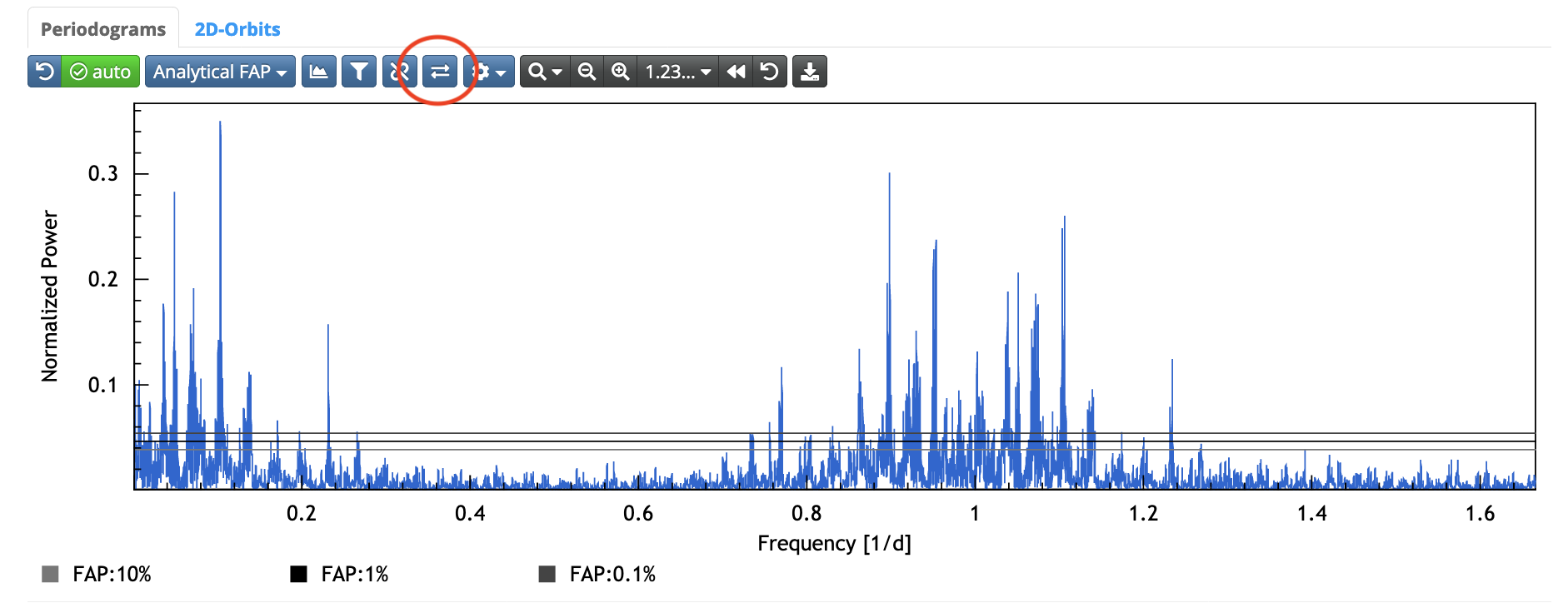
Switch the x axis back and forth beetween periods and frequencies.
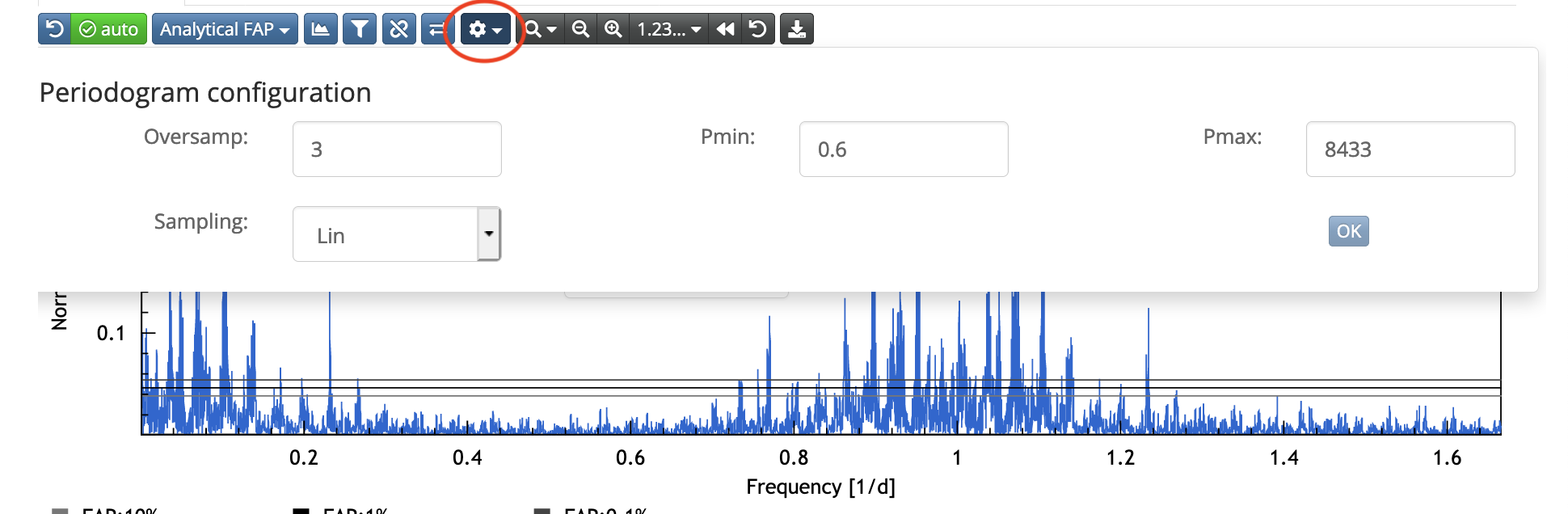
Change the resolution of the periodogram.
Adding a component to your model
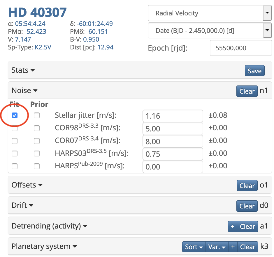
White noise component
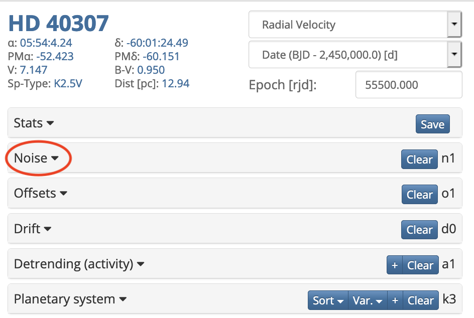
Tick the "fit" box to include a noise term in your model.
Offsets
Each instrument has an offset value that can be fitted.

Drift (polynomial)
You can add a polynomial drift up to order three.

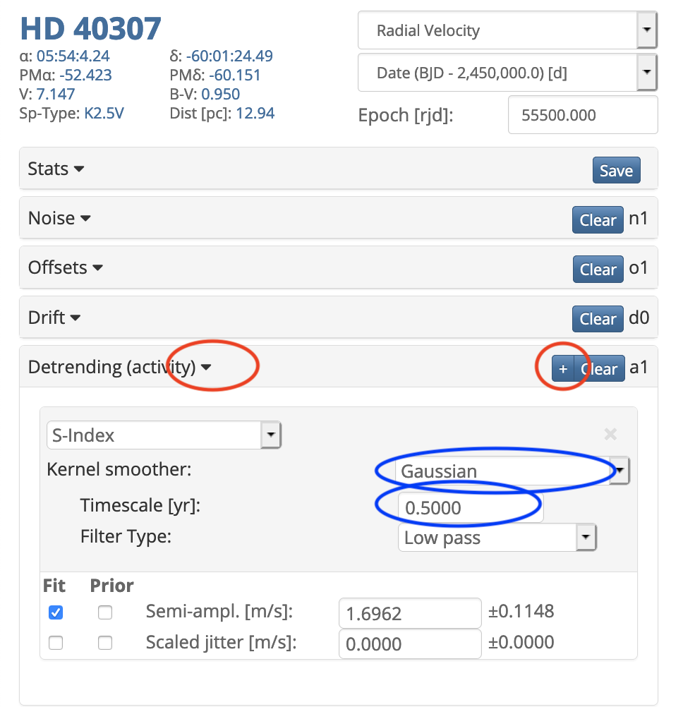
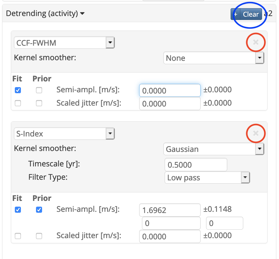
Activity
Add a new activity indicator. Select the smooting kernel and time-scale (in blue).
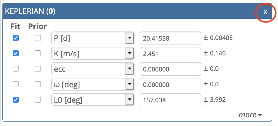
Planet (keplerian signal)
Add a Keplerian signal from the periodogram. Click on the periodogram, then "add a Keplerian".
This will add a Keplerian function to your model whose fit is initialised at the period you selected.
If you want to fit a circular planet
After adding a Keplerian component, set the eccentricity field to 0.
Unselect both eccentricity and argument of periastron.

Deleting a model component
Each planet can be removed from the fit.
The indicators can also bee removed one by one (red) or altogether (blue).
The "clear" icon exists for all model components.
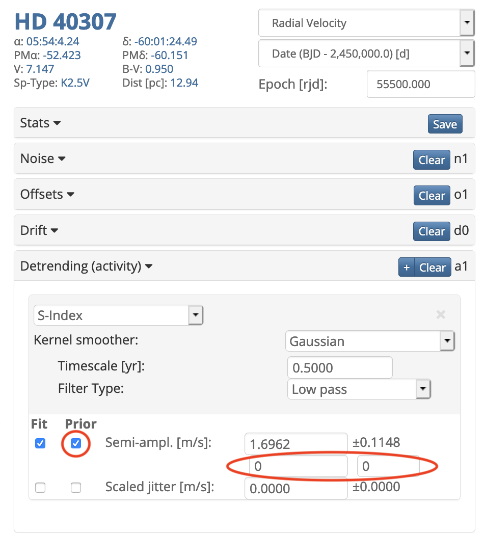
Setting a prior
Tick the box "prior" close to the parameters.
Priors are assumed Gaussian. Within the red ellipse:
the left field is the mean value of the Gaussian, the right field is its standard deviation.
These will be applied to the fit. More general priors can be set for the MCMC analysis (see below).
Fitting parameters
All parameters for which the box "fit" is checked.
Click on the orange "fit" icon, top right.
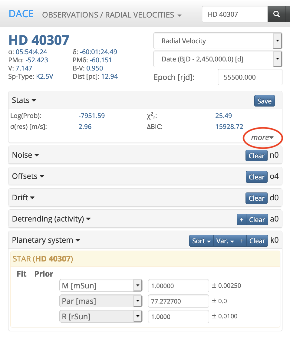
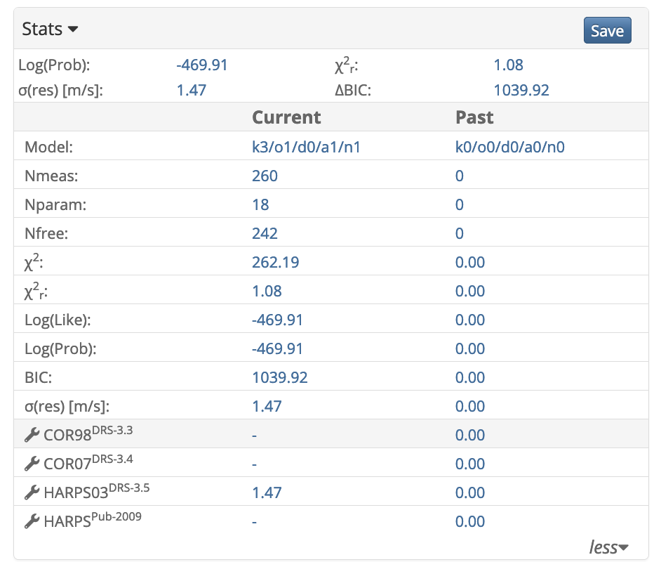
Accessing model statistics
Includes chi squared, Bayesian information criterion (BIC)
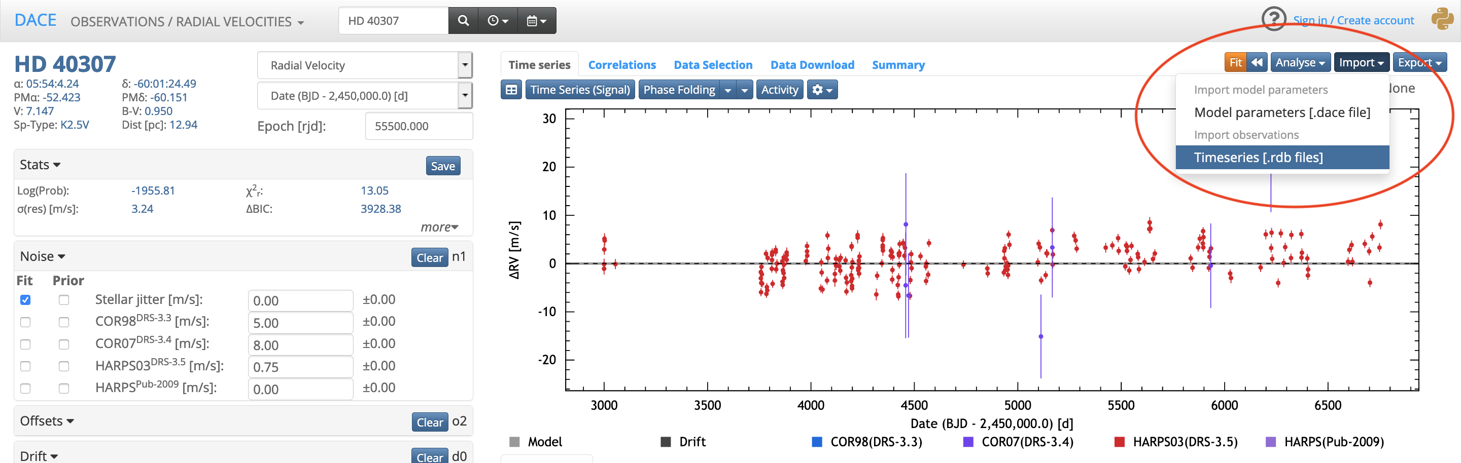
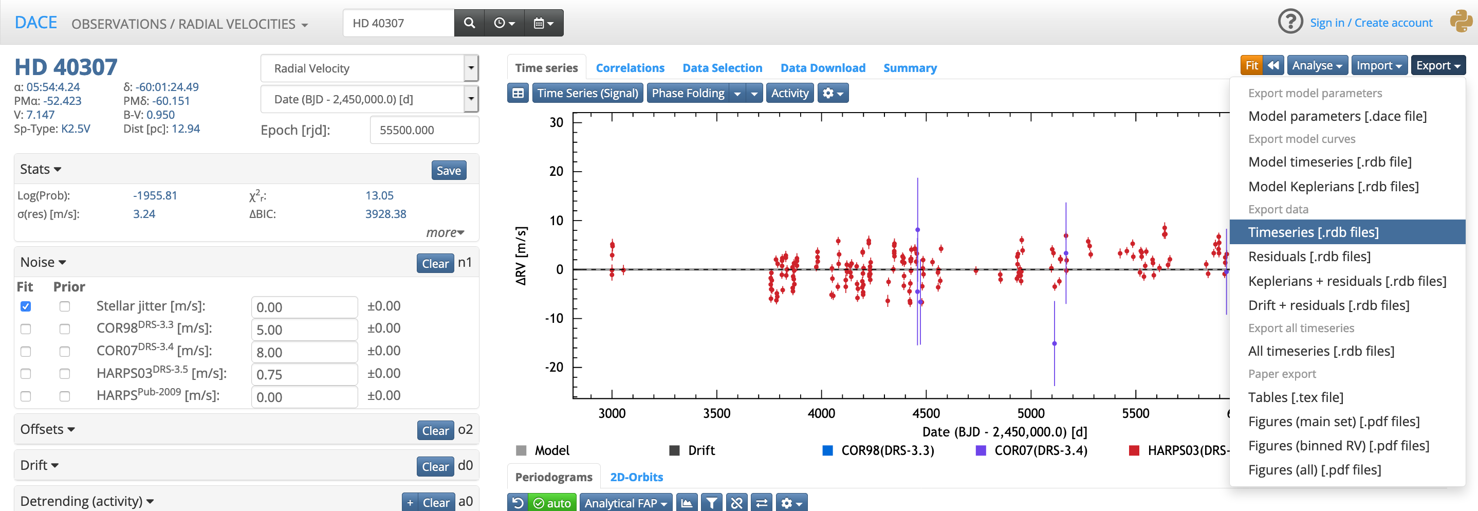
Import/export
Importing your own data.
Exporting the data, the model, etc.
Computing uncertainties with Monte-Carlo Markov chains (MCMC)
For this step,
you will need a Java runtime environment, which you can download for instance
there.
Go to "Analyse", "MCMC"
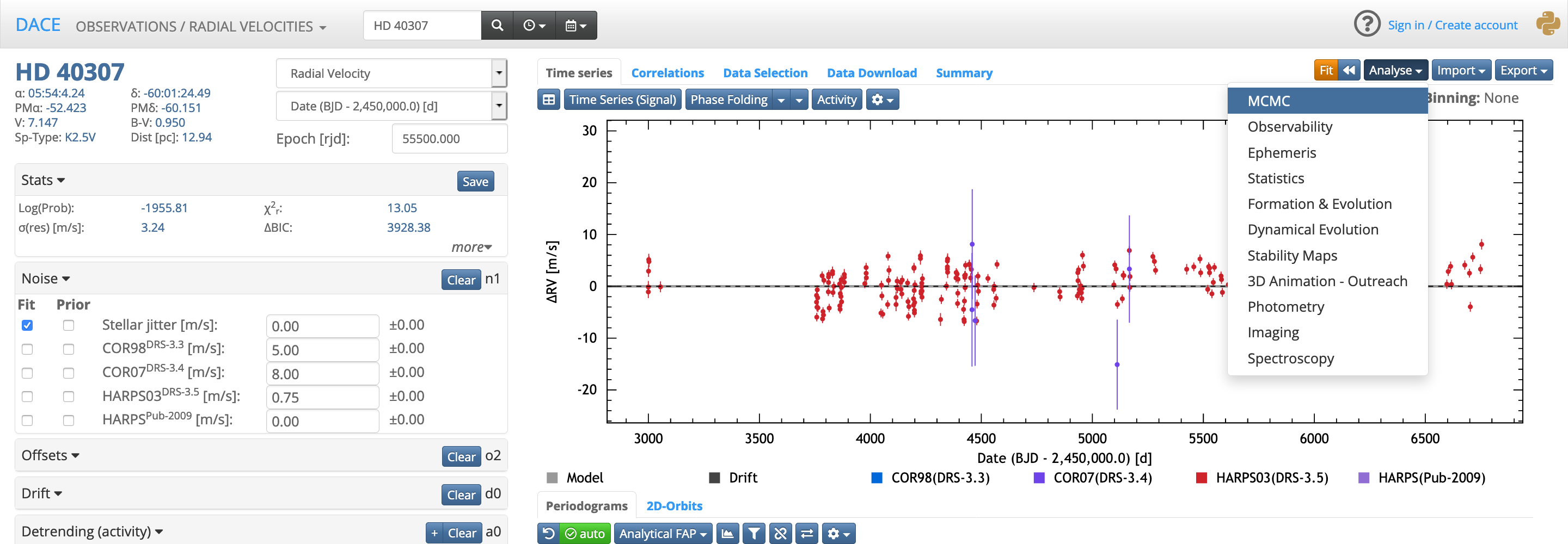
Set your model (already initialised with the parameters for which "fit" is ticked).
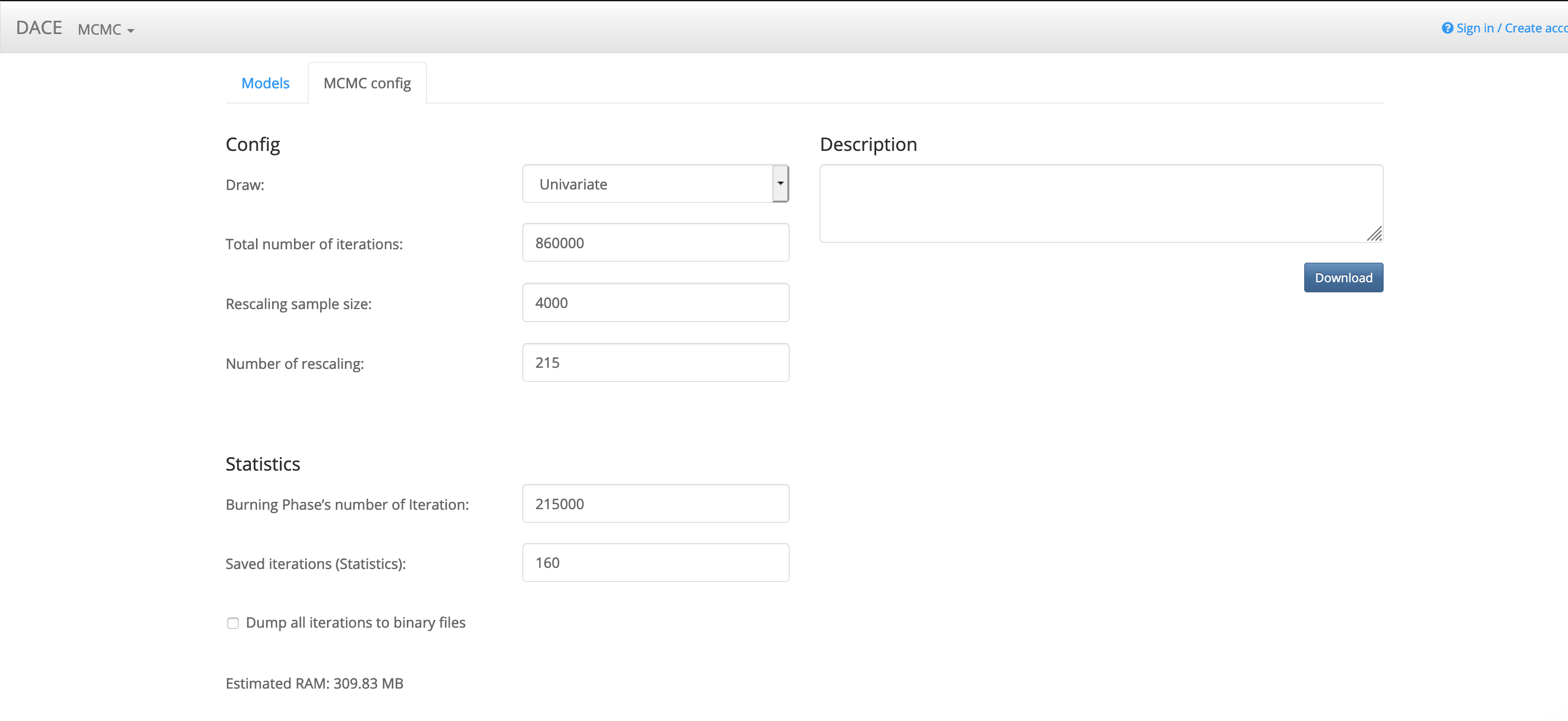
You have several options for the prior.

Select the MCMC parameters (number of iterations in particular).
Click on "Download", to download the MCMC zip file.
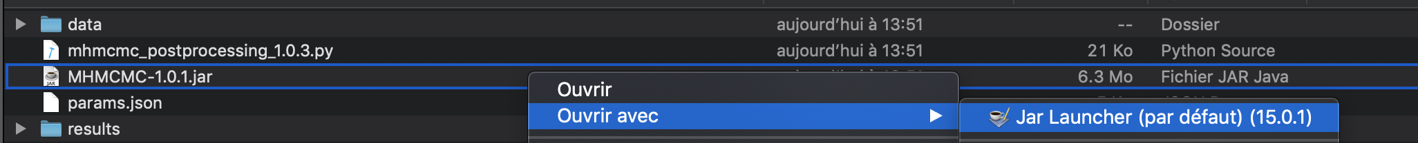
Unzip the file.

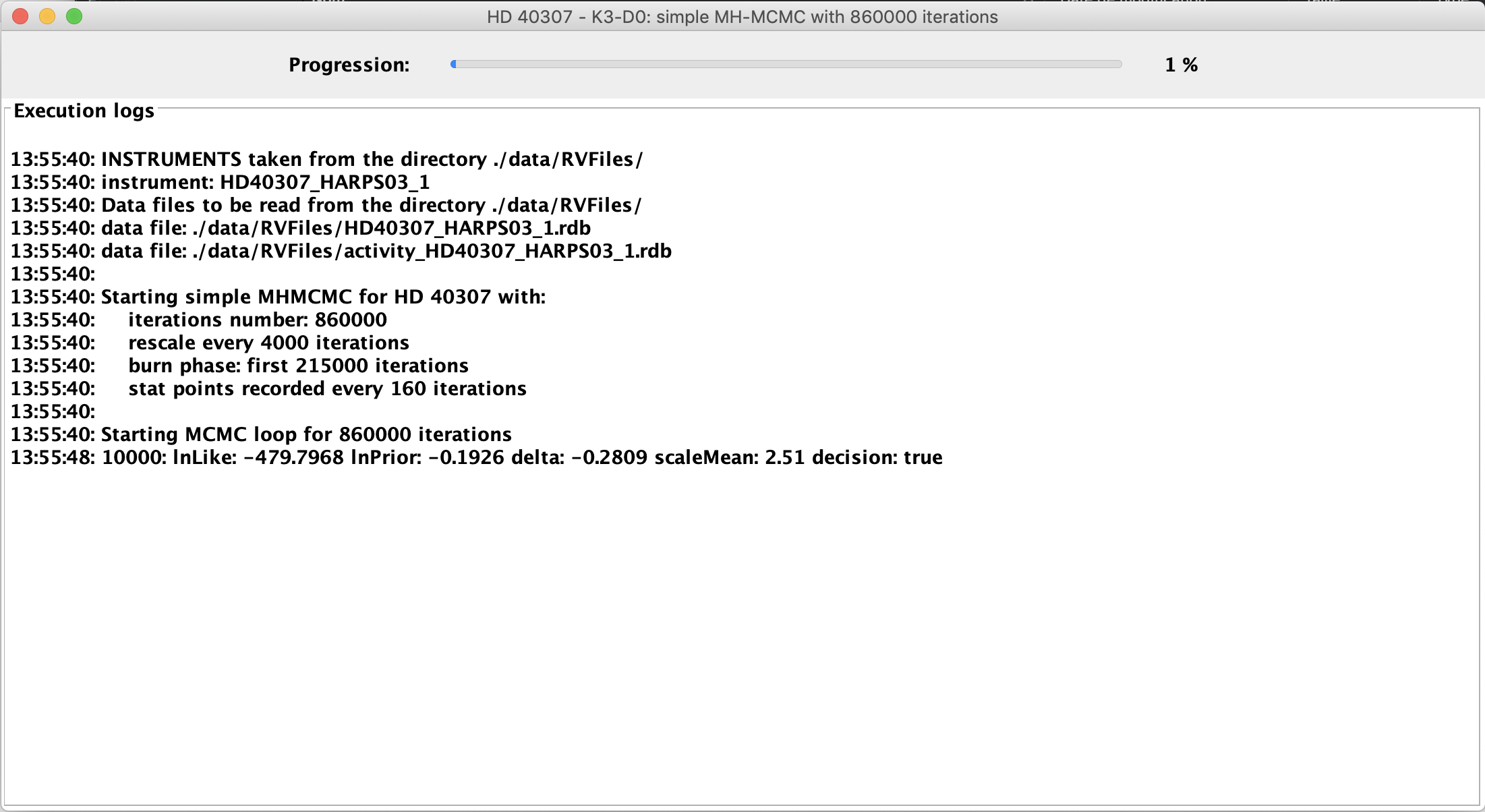
In the folder, open the .jar file with jar launcher.
This will open a window like this:
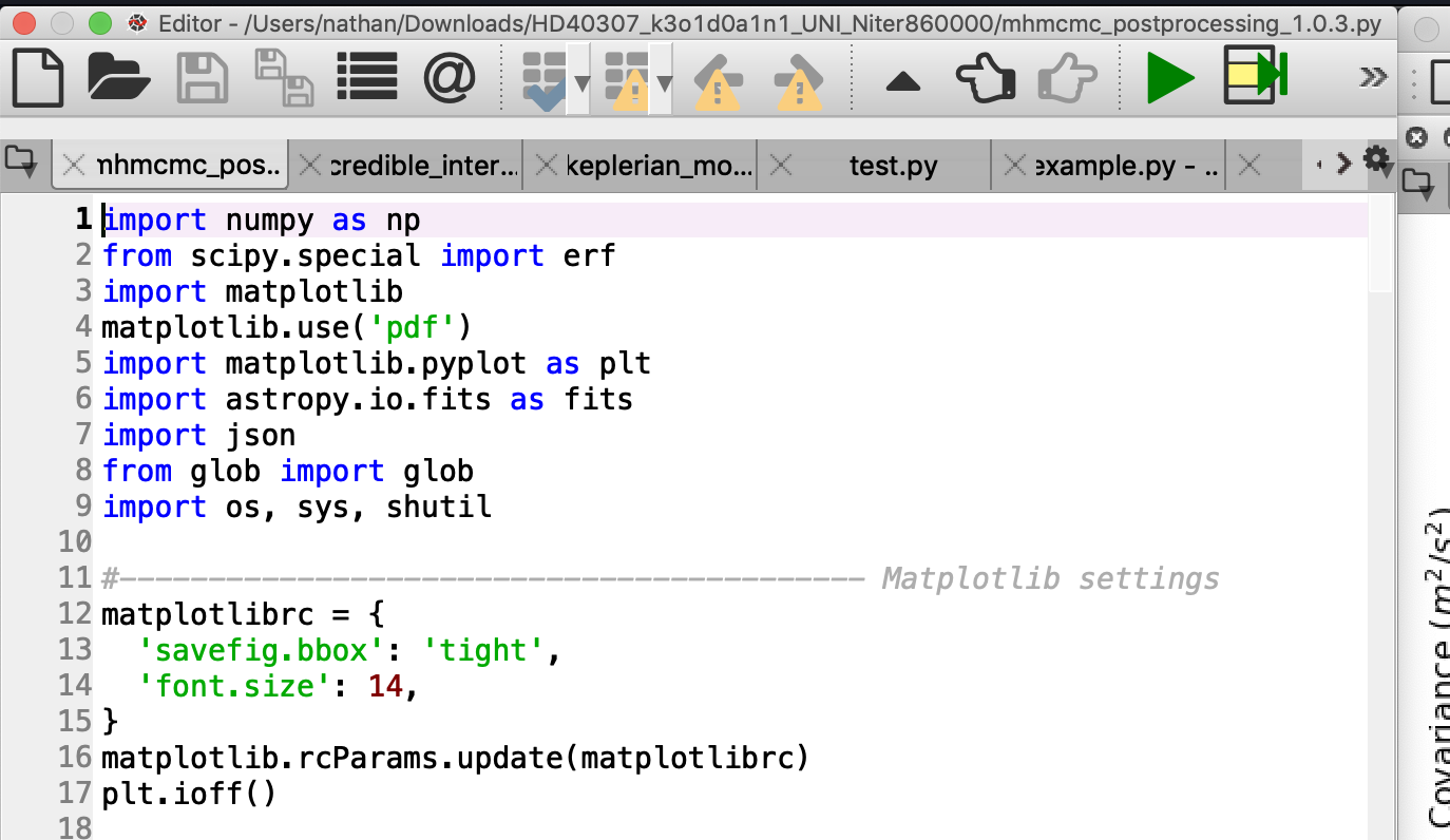
Then execute the .py file, for instance via Spyder:

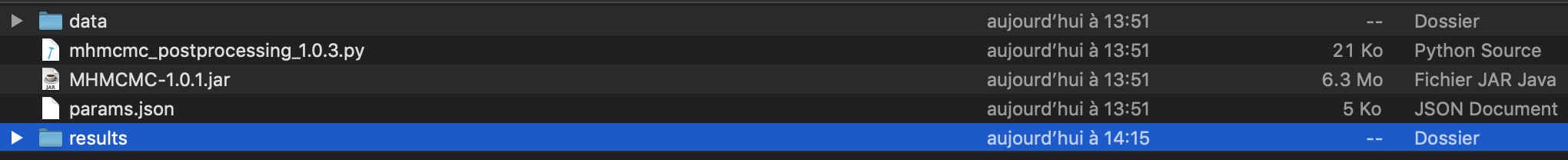
This creates tables and figures that you can access via the following path

For instance, for figures