Exercice 2 - Weighting Galaxies and Clusters of Galaxies
There exist a large number of ways of estimating masses of objects at cosmological distances, such as galaxies and clusters of galaxies. All but one are indirect and model dependent. They rely on the measurement of the radial velocity of different parts of galaxies. We will review these methods, in a much simplified way, and see how another more recent method called gravitational lensing (the deviation of light by massive bodies) can be used as a model-independent way to carry out mass measurements. We will see that both methods are sensitive to dark matter, but gravitational lensing does not need to assume any prior knowledge on how this dark matter is distributed in galaxies to give precise mass measurements.
2.1 - Spiral galaxies and rotating disks
There are essentially two types of galaxies. Elliptical galaxies, that can be seen (at least to the zeroth order) as a “cloud of stars”, and spiral galaxies that include a rotating disk made of stars, dust and gas, and of a bulge that is comparable to a small elliptical galaxy. Both types of galaxies often harbour a central black hole that can be modeled as a point mass given its small size compared with the whole galaxy, and are thought to reside in a large halo of dark matter which precise shape has not been unveiled yet and which is often taken as spherical in most theoretical models of galaxies.
Spectrographs are used to measure the Doppler
velocity shift, either along the long or small axis of the
galaxy. This radial velocity measured at a distance  away
from the center of the galaxy is called the rotation curve. It
is related to the mass contained within a circle of radius . Since
the system is in equilibrium, the centrifugal force seen by a test
particle of mass
away
from the center of the galaxy is called the rotation curve. It
is related to the mass contained within a circle of radius . Since
the system is in equilibrium, the centrifugal force seen by a test
particle of mass  at radius is compensated by the centripetal force (i.e. the
gravitational force):
at radius is compensated by the centripetal force (i.e. the
gravitational force):
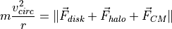
where the three forces involved are produced respectively by the disk,
dark matter halo and central mass components of the galaxy. This
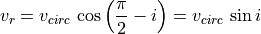
circular velocity  at distance must be multiplied by the
sinus of the inclination
at distance must be multiplied by the
sinus of the inclination  of the spiral along the line of sight
before any comparisons can be made with the observations (Doppler
shifts measure only radial velocities). No measurements can be made of
face-on galaxies since
of the spiral along the line of sight
before any comparisons can be made with the observations (Doppler
shifts measure only radial velocities). No measurements can be made of
face-on galaxies since  in that case.
The gravitational potential generated by the disk
at distance from the galaxy’s center can be expressed as:
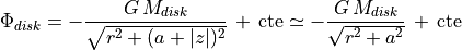
where  is the total mass of the disk,
  is its scale
length, and
is its scale
length, and  is its thickness. We can take
  to make things
easier and since disks in spiral galaxies are very thin.
to make things
easier and since disks in spiral galaxies are very thin.
 is the constant of gravitation.
The potential generated by the dark matter halo is expressed as
a function of its mass density  and its scale length
  :
:
![\Phi_{halo} = 4 \pi G \, \rho_0 \, r_0^2 \, \left\{ \frac{1}{2} \ln\left[1 + \left(\frac{r}{r_0}\right)^2 \right] \,+\,\frac{r_0}{r} \arctan\left(\frac{r}{r_0}\right)\right\} \, + \, \textrm{cte}](../../_images/math/7277a49033bd5e45c659466fd614a862c3ff34d7.png)
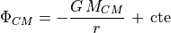
Finally, the potential due to the central mass of the galaxy is given by:
The gravitational force can then be computed from
 .
We will attempt to use this simple three-components model
of the velocity curve of a spiral galaxy to weight it.
.
We will attempt to use this simple three-components model
of the velocity curve of a spiral galaxy to weight it.
First of all, orders of magnitude are necessary and we need to work out the correct units. Based on your knowledge of spiral galaxies, or through the web, try to estimate all the necessary parameters in the model. What are typical sizes for disks, and halos of galaxies ? What are their typical masses ? Estimate, even roughly, the density
of a dark matter halo.
Express in  , the velocity in
  , masses in
 and mass densities in
  .
The mass of the sun is
.
The mass of the sun is  ,
,
 , and
, and
 .
.We will now plot the velocity curve
as a function of the distance from the center.
You can do all this directly in python, using matplotlib.
Plot each of the three components separately for a set of parameters
that spread a plausible range for real galaxies. Plot also the
total velocity . This should help you define which component
(disk, halo, or central mass) is responsible for the “flatness” of the
rotation curve at large .Looking at the image of UGC 111914 estimate roughly the inclination of the disk. Radial velocities have been measured in function of the distance
from the center.
Plot the observed rotation curve of UGC 111914, and estimate all
the model parameters, in order to match the data (knowing that
UGC 111914 lies  away from us). Do not forget the inclination !
First you can simply use gradient descent optimiser such as
away from us). Do not forget the inclination !
First you can simply use gradient descent optimiser such as scipy.optimize.curve_fitto find the best fit.Estimate your uncertainties on each model parameter. To do so, you can run a Markov-Chain Monte-Carlo with the
emceepython package. You will have to introduce some priors on the model parameters and to define the likelihood function. You can complete the code provided with the data. Make sure that your chain has converged. Do you observe degeneracies between the model parameters ? Does this depend on your priors ?What are the masses involved ? You can compute them through numerical integration (
scipy.integrate) of the mass densities, which are given by the Poisson’s law . Remember the coordinates are not cartesian.
What is the total mass of the
galaxy in solar masses ? Approximate its error bars, by computing the total mass for the last 1000 samples
of the chain.
. Remember the coordinates are not cartesian.
What is the total mass of the
galaxy in solar masses ? Approximate its error bars, by computing the total mass for the last 1000 samples
of the chain.
2.2 - Elliptical galaxies as isothermal spheres
Elliptical galaxies are essentially composed of stars and contain very little quantities of gas and dust. Therefore they can be approximated as large clouds of stars. One can see such a system as a gas of particles, where each particle is a star, and where the interaction between the particle is described by the gravitational force. If this system is in a steady state, one gets, by applying statistical mechanics, the following expression (known as a statement of the virial theorem) :

where  is the kinetic energy,
  is the potential energy,
 is the mean-square speed of the system’s stars,
 is the mass of the galaxy, and
  is the gravitational radius.
In many stellar systems, one can approximate
is the gravitational radius.
In many stellar systems, one can approximate  , where
 is the median radius, which is defined to be the radius within which
lies half the system’s mass.
We shall suppose that the considered galaxy has
a nearly spherical symmetry and that the velocity distribution
of the stars is gaussian, then we can express the mean-square speed
in function of the radial velocity dispersion
is the median radius, which is defined to be the radius within which
lies half the system’s mass.
We shall suppose that the considered galaxy has
a nearly spherical symmetry and that the velocity distribution
of the stars is gaussian, then we can express the mean-square speed
in function of the radial velocity dispersion  :
:
Observations show that spectra of elliptical galaxies are very similar to those of red giant stars. And indeed, red giants are known to be the main contributors to the visible light in elliptical galaxies. An interesting point is that the observed absorption lines in the galaxy spectra appear broader than in the stellar spectra. This is simply explained by the fact that the stars are moving around within the galaxy, with velocities that follow a given velocity distribution. Because of this velocities and of the Doppler effect, one observes broadened absorption lines in the galaxy spectra. By examining to which extend these lines are broadened, one can estimate the velocity dispersion in the galaxy, and eventually the mass of the galaxy.
Have a look at the spectrum
 of the K0 III star
and at the spectrum of an elliptical galaxy.
You can do this in python, using the module
of the K0 III star
and at the spectrum of an elliptical galaxy.
You can do this in python, using the module astropy(with the functions inastropy.io.fits) to read the FITS file as well as it’s header, andmatplotlibto draw interactive plots. From the equation of the Doppler shift , one has:
This means that if you want to sample a spectrum linearly in velocity, you have to sample it in function of the logarithm of the wavelength. This is why the
and spectra are sampled in  .
Identify the following important lines in the spectra:
.
Identify the following important lines in the spectra:![\lambda\,[\AA]](../../_images/math/e8a5fb2c4106fea37808d32d042ce42b1e7fa2e4.png)
element
3933.44
Ca, K band
3969.17
Ca, H band
4303.36
CH molecules, G band
4861.32

5174.00
Mg band
5892.36
Na doublet
6562.80

Calculate the sampling of the spectra (i.e. 1 pixel = ? km/s).
If
 is the radial velocity distribution in the galaxy,
one can express the observed galaxy spectrum as the convolution
of the star spectrum with this velocity distribution:
is the radial velocity distribution in the galaxy,
one can express the observed galaxy spectrum as the convolution
of the star spectrum with this velocity distribution:
Determine the radial velocity dispersion
in the galaxy
by supposing that the velocity distribution is gaussian.
You can use the scipy.ndimage.filterspackage which has easy-to-use commands to convolve the stellar spectrum with a gaussian function, which is directly linked to the radial velocity dispersion
(be careful with the units,
is directly linked to the radial velocity dispersion
(be careful with the units, scipy.ndimage.filtersrequires to be expressed in pixels).Try several values of
to estimate which one gives the best
match between and  . This could simply be done
by computing
. This could simply be done
by computing  , and
then examining the results. You can also think of even more advanced possibilities.
, and
then examining the results. You can also think of even more advanced possibilities.From the best-fit radial velocity dispersion estimate the mass of the galaxy (expressed in solar masses) if its gravitational radius is
 .
.
2.3 - Galaxy clusters
One can weight a whole cluster of galaxies in a similar way than we did
for the elliptical galaxy. Whereas, this time, we consider whole
galaxies as our theoretical gas particles, in order to apply the
virial theorem.
Spectroscopy of the galaxies enables us to determine
their mean radial velocities. For a cluster containing  galaxies, the
radial velocity dispersion is then given by:
galaxies, the
radial velocity dispersion is then given by:
where  is the mean radial velocity of the galaxies. From
the radial velocity dispersion you can infer the mass of the cluster.
is the mean radial velocity of the galaxies. From
the radial velocity dispersion you can infer the mass of the cluster.
The redshift of an object is defined as
 .
From the spectra of 20 galaxies of the galaxy cluster
Abell 370, estimate the redshift of each galaxy, and then the
mean redshift of the cluster.
.
From the spectra of 20 galaxies of the galaxy cluster
Abell 370, estimate the redshift of each galaxy, and then the
mean redshift of the cluster.Convert the redshifts into radial velocities. Determine the radial velocity dispersion and the mass of the cluster (
 ).
Given the fact that the cluster contains approximately one hundred
galaxies, what can you conclude about its mass?
).
Given the fact that the cluster contains approximately one hundred
galaxies, what can you conclude about its mass?The measured radial velocities are rather high. Is there any correction we should have thought about, when converting the redshifts into velocities? Or, equivalently, how should radial velocities be computed in a (large enough) comoving volume?