Generating mass profiles

A serie of routines dedictated to the generation of mass profiles are provided by the ic module.

They can be devided according to their geometry:

cubic distribution

function name	description
box	particles in a box

axi-symetrical (disk) distribution

function name	description
homodisk	homogeneous disk
kuzmin	kuzmin disk
expd	exponnential disk
miyamoto_nagai	Miyamoto-Nagai disk

spherical distribution

function name	description
homosphere	homogeneous sphere
plummer	phlummer sphere
nfw	Navarro-Frenk-White profile
hernquist	Hernquist profile
dl2	\[\rho \sim (1-\epsilon (r/r_{\rm{max}})^2)\]
isothm	Isothermal profile
pisothm	Pseudo-Isothermal profile
shell	shell
burkert	Burkert profile
nfwg	Modified Navarro-Frenk-White profile
generic2c	generic two slope model
generic_alpha	\[\rho \sim (r+e)^a\]
generic_Mr	spherical generic model

Finally, some routines generate special object used for rendering:

primer objects

function name	description
line	a simple line
square	a square
circle	a circle
grid	a 2d grid
cube	a cube
sphere	a sphere

Each of these routines returns an Nbody object.

Examples:

>>> from pNbody import ic
>>> nb=ic.box(1000,1,1,1)
>>> nb.info()
-----------------------------------
particle file       : ['box.h5py']
ftype               : 'swift'
mxntpe              : 6
nbody               : 1000
nbody_tot           : 1000
npart               : [1000, 0, 0, 0, 0, 0]
npart_tot           : [1000, 0, 0, 0, 0, 0]
mass_tot            : 1.0000001
byteorder           : 'little'
pio                 : 'no'

len pos : 1000 pos[0] : array([-0.16595599, 0.44064897, -0.99977124], dtype=float32) pos[-1] : array([-0.1209218 , -0.66304606, 0.05817442], dtype=float32) len vel : 1000 vel[0] : array([0., 0., 0.], dtype=float32) vel[-1] : array([0., 0., 0.], dtype=float32) len mass : 1000 mass[0] : 0.001 mass[-1] : 0.001 len num : 1000 num[0] : 0 num[-1] : 999 len tpe : 1000 tpe[0] : 0 tpe[-1] : 0

atime : 0.0 redshift : 0.0 flag_sfr : 0 flag_feedback : 0 flag_cooling : 0 num_files : 1 boxsize : 0.0 omega0 : 0.0 omegalambda : 0.0 hubbleparam : 0.0 flag_age : 0.0 flag_metals : 0.0 nallhw : [0 0 0 0 0 0] critical_energy_spec: 0.0 >>> >>> nb.display()

Generic spherical distributions:

In spherical cases, its possible to generate any mass profile, using a generic function (generic_Mr()). The function takes as argument a vector that defines the cumulative mass as a function of the radius:

\[M(r)=4\pi\int_0^r \rho(r')r'^2 dr'\]

for example, an homogeneous sphere may be obtained by:

>>> from pNbody import ic
>>> import numpy as np
>>> rmax=10
>>> dr=0.01
>>> n = 10000
>>> rs = np.arange(0,rmax,dr)
>>> Mrs = rs**3
>>> nb = ic.generic_Mr(n,rmax=rmax,R=rs,Mr=Mrs,ftype='gadget')

The verctor rs is not necessary linear. This is usefull to avoid resolution problems, if for example, the mass profile is steep in some regions. There, intervals between radial bins may be reduced.

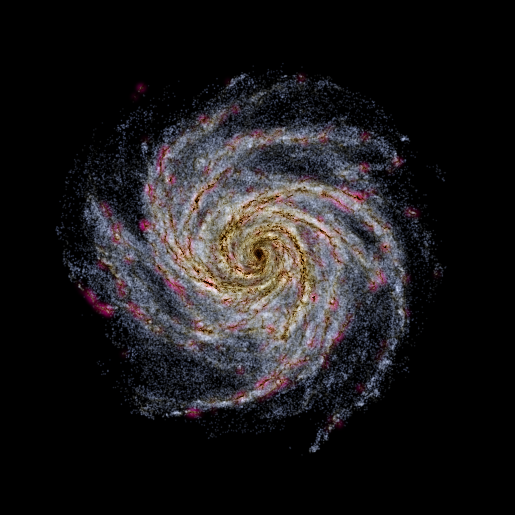
In this more funny example, we generate a radial profile corresponding to the following function:

\[\rho(r) \sim \frac{1}{2}\left[1+\cos(4r) \right] \exp(-r)\]

As before, we use the function generic_Mr():

>>> from pNbody import ic
>>> import numpy as np
>>> n = 1000000
>>> rmax = 10.
>>> dr = 0.01
>>> rs = np.arange(0,rmax,dr)
>>> rho = 0.5*(1+np.cos(4*rs) )*np.exp(-rs)
>>> Mrs = np.add.accumulate(rho*rs**2 * dr)
>>> nb = ic.generic_Mr(n,rmax=rmax,R=rs,Mr=Mrs,ftype='gadget')

It is possible to check the result by extractig the accumulated mass directely from the Nbody object, using the libgrid module:

>>> from pNbody import libgrid
>>> # create a grid object and extract density and mass profile
>>> G = libgrid.Spherical_1d_Grid(rmin=0,rmax=rmax,nr=512,g=None,gm=None)
>>> r  = G.get_r()
>>> rho  = G.get_DensityMap(nb)
>>> mr  = np.add.accumulate(G.get_MassMap(nb))
>>> # plot results
>>> import pylab as pt
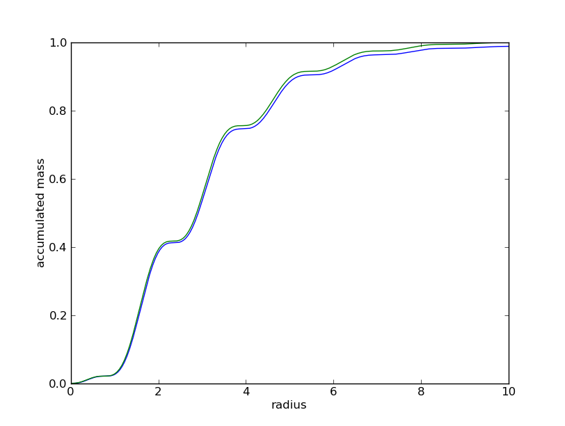
>>> pt.plot(rs,Mrs)
>>> pt.plot(r,mr)
>>> pt.xlabel("radius")
>>> pt.ylabel("accumulated mass")
>>> pt.show()

If everything goes well, we obtain a nice correspondance between the imposed and the computed mass profile, as seen in the graph below.

Generic cubic distributions:

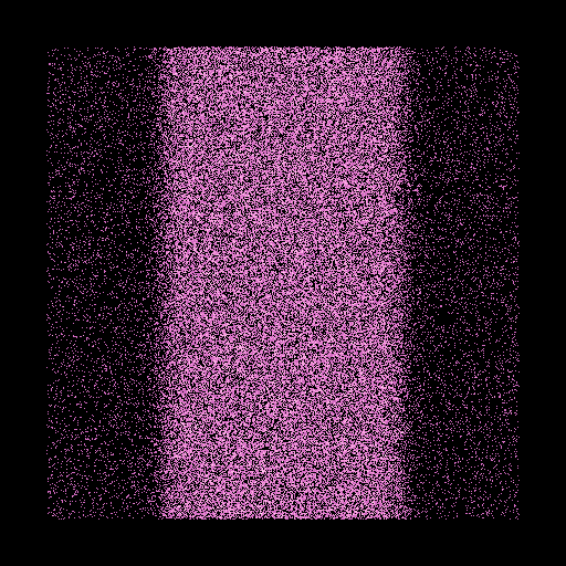
Its possible generate a cubic box with the density varying along one axix. This is obtained by using the generic_Mx() function. As for generic_Mr(), we have to define the variation of the cumulative mass, in this case, the x axis. In the following example, we set a two level transition along the x axis, following the function:

\[\rho(x) = \rho_1 + \frac{\rho_2-\rho_1}{ (1+\exp(-2(x-x_1)/\sigma))(1+\exp(2(x-x_2)/\sigma)) }\]

This gives:

>>> from pNbody import ic
>>> import numpy as np
>>> xs = np.arange(0,1,1./10000.)
>>> n = 100000
>>> rho1 = 1
>>> rho2 = 10
>>> x1 = 0.25
>>> x2 = 0.75
>>> sigma = 0.025
>>> rho = rho1 + (rho2-rho1)/( (1+np.exp(-2.*(xs-x1)/sigma))*(1+np.exp(2.*(xs-x2)/sigma)))
>>> Mxs = np.add.accumulate(rho)
>>> nb = ic.generic_Mx(n,1.0,x=xs,Mx=Mxs,name='tbox.dat',ftype='gadget')

Let’s display now the model:

>>> nb.translate([-0.5,-0.5,-0.5])
>>> nb.show(view='xy',size=(0.6,0.6))

The two density levels are well seen in projection.