Generating velocities
Setting initial velocities may be trivial or very complex, depending on the aim. Of course, its allways possible to directely set the variable ‘’nb.vel’’ to some values. However, in galactic dynamics, this is usually nor the right way to do.
pNbody offers different methods to set the velocities in order to ensure the system to be in a resonably good equilibrium.
method name |
geometry |
method |
|---|---|---|
|
spherical |
jeans equation+self-adaptative grid |
|
spherical |
jeans equation |
|
cylindrical |
jeans equation |
Some examples showing how to set the initial velocities for spherical or axi-symetric models are provided in the example directory. To get it, type:
pNbody_copy-examples
by default, this create a directory in your home ~/pnbody_examples.
The scripts are in the ~/pnbody_examples/ic directory.
Spherical coordinate
In spherical coordinates, supposing that the velocities are isotropics. the Jeans equations is reduced to one integral, giving the value of the velocity dispertion of a component \(i\) :
Example : Set a Plummer sphere to the jeans equilibrium
First, generate the Plummer sphere:
>>> from pNbody import ic
>>> from numpy import *

>>> n = 100000
>>> a = 1.
>>> rmax = 10.
>>> nb = ic.plummer(n,1,1,1,eps=a,rmax=rmax,name='plummer.dat',ftype='gadget')
Then, we need to create a 1D grid wraping the model:
>>> grmin = 0         # grid minimal radius
>>> grmax = rmax*1.05 # grid maximal radius
>>> nr = 128          # number of radial bins
Now, in order to decrease the noise in outer regions, it is usefull to use a non linear grid. In this purpose, we need to define a function that defines the new nodes of the grid. Here, we set it logarithmic. The inverse function is also needed:
>>> rc = a
>>> g  = lambda r:log(r/rc+1)       # the function
>>> gm = lambda r:rc*(exp(r)-1)     # and its inverse
Now it possible to invoque the magic function:
>>> eps = 0.01 # gravitational softening
>>> nb,phi,stats = nb.Get_Velocities_From_Spherical_Grid(eps=eps,nr=nr,rmax=grmax,phi=None,g=g,gm=gm,UseTree=True,ErrTolTheta=0.5)
If UseTree=True the function uses a treecode to compute the potential at each node.
A new nb object with velocities computed from the Jeans equation is returned. We also get the potential in each node
and some statistics. The potential phi is usefull if we need to run the method for another component.
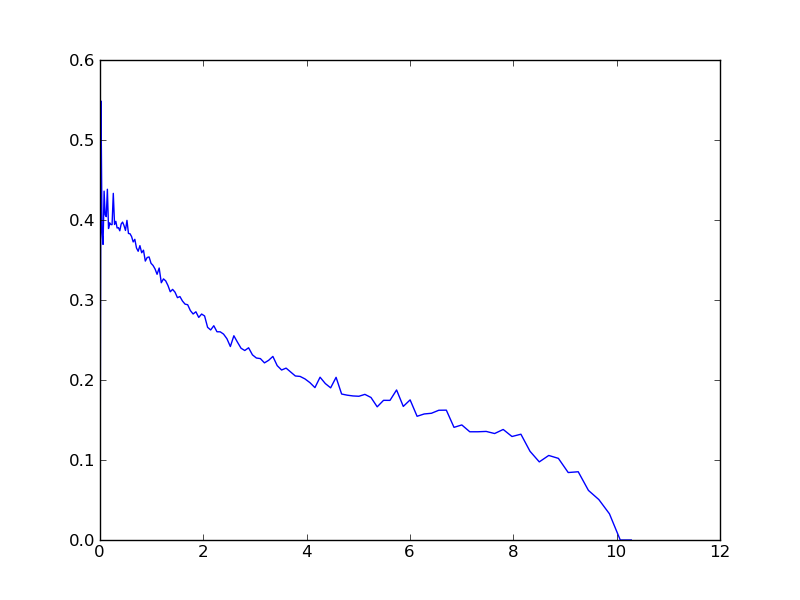
Using the stats variable, it is possible to plot some interesting values used during the computation, like the velocity dispertion as a function of the radius:
>>> import pylab as pt
>>> pt.plot(stats['r'],stats['sigma'])
>>> pt.show()
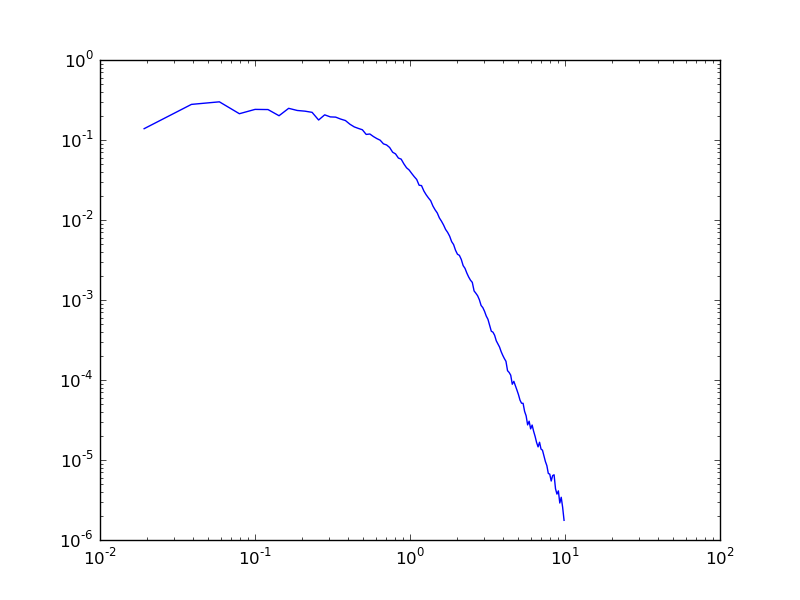
or the density profile:
>>> pt.plot(stats['r'],stats['rho'])
>>> pt.loglog()
>>> pt.show()
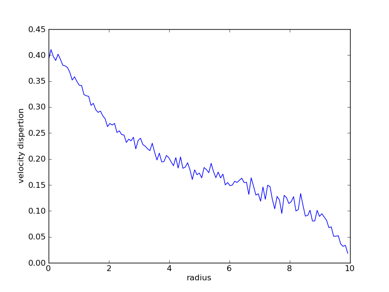
It is possible to check the velocity dispertion along the line of sight directely by mesuring it using a grid object:
>>> from pNbody import libgrid
>>> G = libgrid.Spherical_1d_Grid(rmin=0,rmax=rmax,nr=128,g=None,gm=None)
>>> r   = G.get_r()
>>> sigma = G.get_SigmaValMap(nb,nb.vz())
>>> pt.plot(r,sigma)
>>> pt.xlabel("radius")
>>> pt.ylabel("velocity dispertion")
>>> pt.show()
Cylindrical coordinate
As in spherical geometry, we use the Jeans equations to get an approximation of the velocity dispertions.
Vertical velocity dispersion
The resolution of these equations in cylindrical coordinates gives directely the dispersion along the z axis:
and the mean azimuthal velocity:
Radial velocity dispersion
if
mode_sigma_r['name']='epicyclic_approximation', we use the epicyclic approximation which hold:
the parameter \(\beta^2\) is set by the variable mode_sigma_r['param'] and takes usually a value around 1.
if
mode_sigma_r['name']='isothropic', the value is simply:
if
mode_sigma_r['name']='toomre', we determine the velocity dispersion uses the Safronov-Toomre parameter \(Q\):\[\sigma_R = \frac{3.36 Q G \Sigma_i}{\kappa}\]\(Q\) is set with the variable
mode_sigma_r['param'].if
mode_sigma_r['name']='constant', the value is simply constant, given by the variablemode_sigma_r['param']:
Azimuthal velocity dispersion
if
mode_sigma_p['name']='epicyclic_approximation', we use the epicyclic approximation which hold:
if
mode_sigma_p['name']='isothropic', the value is simply:
Mean azimuthal velocity
Finally, the mean azimuthal velocity is also derived directely from the Jeans equations:
Example : Set an exponnential disk to the jeans equilibrium
Lest try to put an exponnential disk at the Jeans equilibrium. First, we generate the disk:
>>> from pNbody import ic
>>> from numpy import *
>>> n = 100000
>>> Hz = 0.3
>>> Hr = 3.
>>> Rmax = 30.
>>> Zmax = 3.
>>> nb = ic.expd(n,Hr,Hz,Rmax,Zmax,irand=1,name='expd.dat',ftype='gadget')
Then, we need to set the parameters for the cylindrical grid:
>>> grmin        = 0.            # minimal grid radius
>>> grmax        =  1.1*Rmax     # maximal grid radius
>>> gzmin        = -1.1*Zmax     # minimal grid z
>>> gzmax        =  1.1*Zmax     # maximal grid z
>>> nr           = 32            # number of bins in r
>>> nt           = 2             # number of bins in t
>>> nz           = 64+1          # number of bins in z
- Set some functions used to distort the grid along the radius::
>>> rc           = Hr
>>> g            = lambda r:log(r/rc+1.)
>>> gm           = lambda r:rc*(exp(r)-1.)
Set some options on how to compute velocity dispertions:
>>> mode_sigma_z = {"name":"jeans","param":None}
>>> mode_sigma_r = {"name":"toomre","param":1.0}
>>> mode_sigma_p = {"name":"epicyclic_approximation","param":None}
>>> params = [mode_sigma_z,mode_sigma_r,mode_sigma_p]
Set the gravitational softening:
>>> eps=0.1
And finally, lunch the magic function:
>>> nb,phi,stats = nb.Get_Velocities_From_Cylindrical_Grid(select='0',disk=(0),eps=eps,nR=nr,nz=nz,nt=nt,Rmax=grmax,zmin=gzmin,zmax=gzmax,params=params,Phi=None,g=g,gm=gm)
The parameter select='0' tells that we want to compute the velocities on particles of type 0, while
disk=0 tells that what we considere as the disk is only the particles 0. This is usefull when dealing with
multi-component models.
The latter function return nb with the new velocities, a matrix phi containing the potential at each node of the grid,
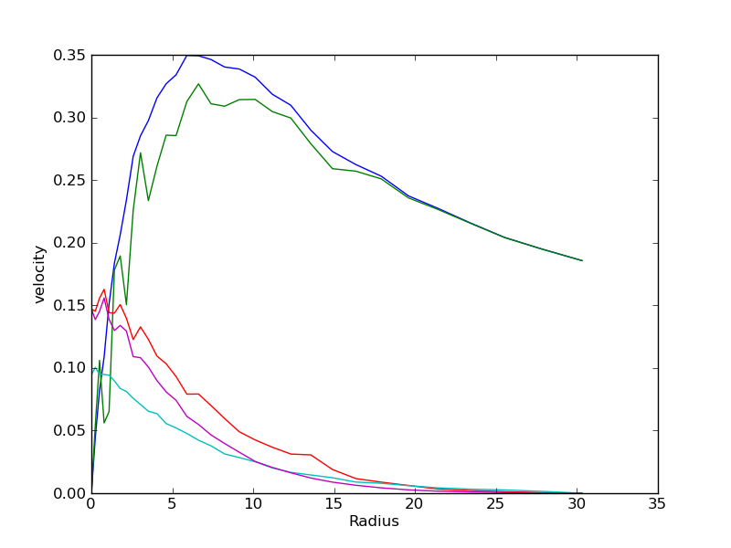
and a dictrionary stats containing some physical usefull quantities. Lets plot some of them:
>>> import pylab as pt
>>> pt.plot(stats['R'],stats['vc'])
>>> pt.plot(stats['R'],stats['vm'])
>>> pt.plot(stats['R'],stats['sr'])
>>> pt.plot(stats['R'],stats['sz'])
>>> pt.plot(stats['R'],stats['sp'])
>>> pt.xlabel('Radius')
>>> pt.ylabel('velocity')
>>> pt.show()
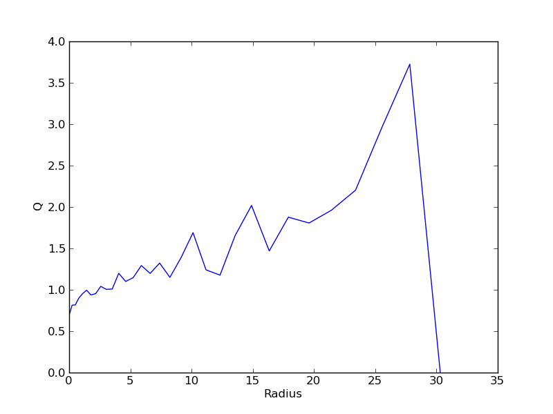
Lets try instead of fixing the Tomre parameter, to use for the radial velocity dispertion the epicyclic approximation. This is done by using the following parameters:
>>> mode_sigma_z = {"name":"jeans","param":None}
>>> mode_sigma_r = {"name":"epicyclic_approximation","param":1}
>>> mode_sigma_p = {"name":"epicyclic_approximation","param":None}
>>> params = [mode_sigma_z,mode_sigma_r,mode_sigma_p]
again, run the magic function:
>>> nb,phi,stats = nb.Get_Velocities_From_Cylindrical_Grid(select='0',disk=(0),eps=eps,nR=nr,nz=nz,nt=nt,Rmax=grmax,zmin=gzmin,zmax=gzmax,params=params,Phi=None,g=g,gm=gm)
Now lets plot the Tommre parameter:
>>> pt.plot(stats['R'],stats['Q'])
>>> pt.xlabel('Radius')
>>> pt.ylabel('Q')
>>> pt.show()
Multi component systems
Examples using multicomponents systems are provided in the pnbody_examples/ic directory obtained
with the command:
pNbody_copy-examples