Matplotlib (Python3) tutorial

• official website : http://matplotlib.org/
• examples : https://matplotlib.org/tutorials/introductory/sample_plots.html
• gallery : https://matplotlib.org/gallery/index.html

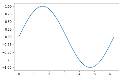
A tutorial in 6 lines

import numpy as np
import pylab as plt
x = np.linspace(0,2*np.pi,100)
y = np.sin(x)
plt.plot(x,y)
plt.show()

Slightly more complete example

import numpy as np
import pylab as plt
x = np.linspace(0,2*np.pi,100)
y = np.sin(x)
z = np.cos(x)
plt.plot(x,y)
plt.plot(x,z)
plt.plot(x,y,'-r')
plt.plot(x,z,'.b')
plt.scatter(x,y)
plt.xlabel("x")
plt.ylabel("y,z")
plt.title("A tutorial in one example")
plt.show()

Other useful plot types

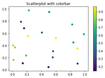
Scatterplots: When different points have different values

import numpy as np
import pylab as plt
# create some random values to plot
x = np.random.uniform(size=20) # creates an array containing 20 random numbers between [0,1) following an uniform PDF
y = np.random.uniform(size=20)
vals = np.random.uniform(size=20)
scp = plt.scatter(x, y,       # x and y values of points
                  c=vals      # values that determine the colours of the points
                 )
plt.colorbar()
plt.title("Scatterplot with colorbar")
plt.xlabel("x")
plt.ylabel("y")
plt.show()

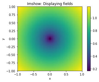
Imshow: Displaying a field

import numpy as np
import pylab as plt

nx = 50    # number of plot points
xmin = -1  # lower bound for plot
xmax = 1   # upper bound for plot
dx = (xmax - xmin)/nx # cell size

# invent some data
data = np.zeros((nx, nx), dtype=np.float)
for i in range(nx):
    for j in range(nx):
        xx = xmin + (i+0.5)*dx # cell centre
        yy = xmin + (j+0.5)*dx
        data[j,i] = 1./np.sqrt(1./np.sqrt(xx**2 + yy**2))

# data[j, i] is no accident. The plotting function, imshow(), assumes that the image
# is given as an m x n array, and will plot the indices [0, 0] in the upper left corner
# and [m-1, n-1] at the bottom right corner, where m is the height of the image and
# n the width; So opposite of what we're used to from (x, y) coordinates.


scp = plt.imshow(data,    #which data to plot
                 extent=(xmin, xmax, xmin, xmax), # set plot limits. If not set, imshow will label cell numbers.
                 origin='lower' # start the image plotting from below, not from above
                )


plt.colorbar()
plt.title("Imshow: Displaying fields")
plt.xlabel("x")
plt.ylabel("y")
plt.show()

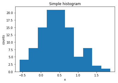
Histogramming

import matplotlib.pyplot as plt
import numpy as np



# define some data
data = np.random.normal(0.5, 0.5, 100) # 100 samples of normal (Gaussian) distribution around 0.5 with sigma=0.5

plt.hist(data,      # data to plot
        bins=10,    # how many bins to use; or give an array of bin edges
        cumulative=False
        )

plt.title("Simple histogram")
plt.xlabel("x")
plt.ylabel("counts")
plt.show()