Scipy (Python3) tutorial

• official website : http://www.scipy.org/
• documentation : https://docs.scipy.org/doc/scipy/reference/
• Tutorial : https://docs.scipy.org/doc/scipy/reference/tutorial/index.html

Packages

Topic	package name
Special functions	scipy.special
Integration	scipy.integrate
Optimization	scipy.optimize
Interpolation	scipy.interpolate
Fourier Transforms	scipy.fftpack
Signal Processing	scipy.signal
Linear Algebra	scipy.linalg
Sparse Eigenvalue Problems with ARPACK	scipy.sparse.linalg
Compressed Sparse Graph Routines	scipy.sparse.csgraph
Spatial data structures and algorithms	scipy.spatial
Statistics	scipy.stats
Multidimensional image processing	scipy.ndimage
File IO	scipy.io

Integration

Load modules:

import numpy as np
from scipy import integrate

help:

help(integrate.quad)

Help on function quad in module scipy.integrate.quadpack:

quad(func, a, b, args=(), full_output=0, epsabs=1.49e-08, epsrel=1.49e-08, limit=50, points=None, weight=None, wvar=None, wopts=None, maxp1=50, limlst=50)
    Compute a definite integral.

    Integrate func from `a` to `b` (possibly infinite interval) using a
    technique from the Fortran library QUADPACK.

    Parameters
    ----------
    func : {function, scipy.LowLevelCallable}
        A Python function or method to integrate.  If `func` takes many
        arguments, it is integrated along the axis corresponding to the
        first argument.

        If the user desires improved integration performance, then `f` may
        be a `scipy.LowLevelCallable` with one of the signatures::

            double func(double x)
            double func(double x, void *user_data)
            double func(int n, double *xx)
            double func(int n, double *xx, void *user_data)

        The ``user_data`` is the data contained in the `scipy.LowLevelCallable`.
        In the call forms with ``xx``,  ``n`` is the length of the ``xx``
        array which contains ``xx[0] == x`` and the rest of the items are
        numbers contained in the ``args`` argument of quad.

        In addition, certain ctypes call signatures are supported for
        backward compatibility, but those should not be used in new code.
    a : float
        Lower limit of integration (use -numpy.inf for -infinity).
    b : float
        Upper limit of integration (use numpy.inf for +infinity).
    args : tuple, optional
        Extra arguments to pass to `func`.
    full_output : int, optional
        Non-zero to return a dictionary of integration information.
        If non-zero, warning messages are also suppressed and the
        message is appended to the output tuple.

    Returns
    -------
    y : float
        The integral of func from `a` to `b`.
    abserr : float
        An estimate of the absolute error in the result.
    infodict : dict
        A dictionary containing additional information.
        Run scipy.integrate.quad_explain() for more information.
    message
        A convergence message.
    explain
        Appended only with 'cos' or 'sin' weighting and infinite
        integration limits, it contains an explanation of the codes in
        infodict['ierlst']

    Other Parameters
    ----------------
    epsabs : float or int, optional
        Absolute error tolerance.
    epsrel : float or int, optional
        Relative error tolerance.
    limit : float or int, optional
        An upper bound on the number of subintervals used in the adaptive
        algorithm.
    points : (sequence of floats,ints), optional
        A sequence of break points in the bounded integration interval
        where local difficulties of the integrand may occur (e.g.,
        singularities, discontinuities). The sequence does not have
        to be sorted.
    weight : float or int, optional
        String indicating weighting function. Full explanation for this
        and the remaining arguments can be found below.
    wvar : optional
        Variables for use with weighting functions.
    wopts : optional
        Optional input for reusing Chebyshev moments.
    maxp1 : float or int, optional
        An upper bound on the number of Chebyshev moments.
    limlst : int, optional
        Upper bound on the number of cycles (>=3) for use with a sinusoidal
        weighting and an infinite end-point.

    See Also
    --------
    dblquad : double integral
    tplquad : triple integral
    nquad : n-dimensional integrals (uses `quad` recursively)
    fixed_quad : fixed-order Gaussian quadrature
    quadrature : adaptive Gaussian quadrature
    odeint : ODE integrator
    ode : ODE integrator
    simps : integrator for sampled data
    romb : integrator for sampled data
    scipy.special : for coefficients and roots of orthogonal polynomials

    Notes
    -----

    **Extra information for quad() inputs and outputs**

    If full_output is non-zero, then the third output argument
    (infodict) is a dictionary with entries as tabulated below.  For
    infinite limits, the range is transformed to (0,1) and the
    optional outputs are given with respect to this transformed range.
    Let M be the input argument limit and let K be infodict['last'].
    The entries are:

    'neval'
        The number of function evaluations.
    'last'
        The number, K, of subintervals produced in the subdivision process.
    'alist'
        A rank-1 array of length M, the first K elements of which are the
        left end points of the subintervals in the partition of the
        integration range.
    'blist'
        A rank-1 array of length M, the first K elements of which are the
        right end points of the subintervals.
    'rlist'
        A rank-1 array of length M, the first K elements of which are the
        integral approximations on the subintervals.
    'elist'
        A rank-1 array of length M, the first K elements of which are the
        moduli of the absolute error estimates on the subintervals.
    'iord'
        A rank-1 integer array of length M, the first L elements of
        which are pointers to the error estimates over the subintervals
        with ``L=K`` if ``K<=M/2+2`` or ``L=M+1-K`` otherwise. Let I be the
        sequence ``infodict['iord']`` and let E be the sequence
        ``infodict['elist']``.  Then ``E[I[1]], ..., E[I[L]]`` forms a
        decreasing sequence.

    If the input argument points is provided (i.e. it is not None),
    the following additional outputs are placed in the output
    dictionary.  Assume the points sequence is of length P.

    'pts'
        A rank-1 array of length P+2 containing the integration limits
        and the break points of the intervals in ascending order.
        This is an array giving the subintervals over which integration
        will occur.
    'level'
        A rank-1 integer array of length M (=limit), containing the
        subdivision levels of the subintervals, i.e., if (aa,bb) is a
        subinterval of ``(pts[1], pts[2])`` where ``pts[0]`` and ``pts[2]``
        are adjacent elements of ``infodict['pts']``, then (aa,bb) has level l
        if ``|bb-aa| = |pts[2]-pts[1]| * 2**(-l)``.
    'ndin'
        A rank-1 integer array of length P+2.  After the first integration
        over the intervals (pts[1], pts[2]), the error estimates over some
        of the intervals may have been increased artificially in order to
        put their subdivision forward.  This array has ones in slots
        corresponding to the subintervals for which this happens.

    **Weighting the integrand**

    The input variables, *weight* and *wvar*, are used to weight the
    integrand by a select list of functions.  Different integration
    methods are used to compute the integral with these weighting
    functions.  The possible values of weight and the corresponding
    weighting functions are.

    ==========  ===================================   =====================
    ``weight``  Weight function used                  ``wvar``
    ==========  ===================================   =====================
    'cos'       cos(w*x)                              wvar = w
    'sin'       sin(w*x)                              wvar = w
    'alg'       g(x) = ((x-a)**alpha)*((b-x)**beta)   wvar = (alpha, beta)
    'alg-loga'  g(x)*log(x-a)                         wvar = (alpha, beta)
    'alg-logb'  g(x)*log(b-x)                         wvar = (alpha, beta)
    'alg-log'   g(x)*log(x-a)*log(b-x)                wvar = (alpha, beta)
    'cauchy'    1/(x-c)                               wvar = c
    ==========  ===================================   =====================

    wvar holds the parameter w, (alpha, beta), or c depending on the weight
    selected.  In these expressions, a and b are the integration limits.

    For the 'cos' and 'sin' weighting, additional inputs and outputs are
    available.

    For finite integration limits, the integration is performed using a
    Clenshaw-Curtis method which uses Chebyshev moments.  For repeated
    calculations, these moments are saved in the output dictionary:

    'momcom'
        The maximum level of Chebyshev moments that have been computed,
        i.e., if ``M_c`` is ``infodict['momcom']`` then the moments have been
        computed for intervals of length ``|b-a| * 2**(-l)``,
        ``l=0,1,...,M_c``.
    'nnlog'
        A rank-1 integer array of length M(=limit), containing the
        subdivision levels of the subintervals, i.e., an element of this
        array is equal to l if the corresponding subinterval is
        ``|b-a|* 2**(-l)``.
    'chebmo'
        A rank-2 array of shape (25, maxp1) containing the computed
        Chebyshev moments.  These can be passed on to an integration
        over the same interval by passing this array as the second
        element of the sequence wopts and passing infodict['momcom'] as
        the first element.

    If one of the integration limits is infinite, then a Fourier integral is
    computed (assuming w neq 0).  If full_output is 1 and a numerical error
    is encountered, besides the error message attached to the output tuple,
    a dictionary is also appended to the output tuple which translates the
    error codes in the array ``info['ierlst']`` to English messages.  The
    output information dictionary contains the following entries instead of
    'last', 'alist', 'blist', 'rlist', and 'elist':

    'lst'
        The number of subintervals needed for the integration (call it ``K_f``).
    'rslst'
        A rank-1 array of length M_f=limlst, whose first ``K_f`` elements
        contain the integral contribution over the interval
        ``(a+(k-1)c, a+kc)`` where ``c = (2*floor(|w|) + 1) * pi / |w|``
        and ``k=1,2,...,K_f``.
    'erlst'
        A rank-1 array of length ``M_f`` containing the error estimate
        corresponding to the interval in the same position in
        ``infodict['rslist']``.
    'ierlst'
        A rank-1 integer array of length ``M_f`` containing an error flag
        corresponding to the interval in the same position in
        ``infodict['rslist']``.  See the explanation dictionary (last entry
        in the output tuple) for the meaning of the codes.

    Examples
    --------
    Calculate :math:`\int^4_0 x^2 dx` and compare with an analytic result

    >>> from scipy import integrate
    >>> x2 = lambda x: x**2
    >>> integrate.quad(x2, 0, 4)
    (21.333333333333332, 2.3684757858670003e-13)
    >>> print(4**3 / 3.)  # analytical result
    21.3333333333

    Calculate :math:`\int^\infty_0 e^{-x} dx`

    >>> invexp = lambda x: np.exp(-x)
    >>> integrate.quad(invexp, 0, np.inf)
    (1.0, 5.842605999138044e-11)

    >>> f = lambda x,a : a*x
    >>> y, err = integrate.quad(f, 0, 1, args=(1,))
    >>> y
    0.5
    >>> y, err = integrate.quad(f, 0, 1, args=(3,))
    >>> y
    1.5

    Calculate :math:`\int^1_0 x^2 + y^2 dx` with ctypes, holding
    y parameter as 1::

        testlib.c =>
            double func(int n, double args[n]){
                return args[0]*args[0] + args[1]*args[1];}
        compile to library testlib.*

    ::

       from scipy import integrate
       import ctypes
       lib = ctypes.CDLL('/home/.../testlib.*') #use absolute path
       lib.func.restype = ctypes.c_double
       lib.func.argtypes = (ctypes.c_int,ctypes.c_double)
       integrate.quad(lib.func,0,1,(1))
       #(1.3333333333333333, 1.4802973661668752e-14)
       print((1.0**3/3.0 + 1.0) - (0.0**3/3.0 + 0.0)) #Analytic result
       # 1.3333333333333333

Methods for Integrating Functions given function object:

integrate.quad(np.cos,0,np.pi/2.)

(0.9999999999999999, 1.1102230246251564e-14)

Methods for Integrating Functions given fixed samples:

x = np.arange(0,np.pi/2.,np.pi/100.)
y = np.cos(x)

integrate using the trapeze method:

integrate.trapz(y,x)

0.99942435289390408

integrate using the simpson method:

integrate.simps(y,x)

0.99950521309271656

Optimization

Load module:

from scipy.optimize import leastsq

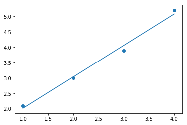
Fit a linear regression to data

start wiith some data:

x = np.array([1,2,3,4],float)
y = np.array([2.1,3,3.9,5.2],float)

define a fitting function:

def linfct(x,a,b):
  return a*x + b

define a residual function

def residuals(p, x, y):
  a,b = p
  err = y-linfct(x,a,b)
  return err

first guess

p0 = 1.,1.

find optimal values

plsq,cmt = leastsq(residuals, p0, args=(x, y))
a = plsq[0]
b = plsq[1]
a,b

(1.0200000000000435, 1.0)

compute the fit

yf = linfct(x,a,b)

now, plot:

import pylab as plt
plt.scatter(x,y)
plt.plot(x,yf)
plt.show()

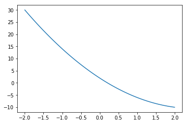
Root finding routines

Define a function

def f(x):
  return 2*x*x - 10*x + 2

import pylab as plt
x = np.linspace(-2,2,50)
plt.plot(x,f(x))
plt.show()

Using the Newtown method to solve

from scipy.optimize import newton
x0 = 0
newton(f,x0)

0.20871215252207997

Using the Bissection method

from scipy.optimize import bisect
xmin=-2
xmax=2
bisect(f,xmin,xmax)

0.20871215252373077

Interpolation

Load module

from scipy import interpolate

help(interpolate.splrep)

Help on function splrep in module scipy.interpolate.fitpack:

splrep(x, y, w=None, xb=None, xe=None, k=3, task=0, s=None, t=None, full_output=0, per=0, quiet=1)
    Find the B-spline representation of 1-D curve.

    Given the set of data points ``(x[i], y[i])`` determine a smooth spline
    approximation of degree k on the interval ``xb <= x <= xe``.

    Parameters
    ----------
    x, y : array_like
        The data points defining a curve y = f(x).
    w : array_like, optional
        Strictly positive rank-1 array of weights the same length as x and y.
        The weights are used in computing the weighted least-squares spline
        fit. If the errors in the y values have standard-deviation given by the
        vector d, then w should be 1/d. Default is ones(len(x)).
    xb, xe : float, optional
        The interval to fit.  If None, these default to x[0] and x[-1]
        respectively.
    k : int, optional
        The degree of the spline fit. It is recommended to use cubic splines.
        Even values of k should be avoided especially with small s values.
        1 <= k <= 5
    task : {1, 0, -1}, optional
        If task==0 find t and c for a given smoothing factor, s.

        If task==1 find t and c for another value of the smoothing factor, s.
        There must have been a previous call with task=0 or task=1 for the same
        set of data (t will be stored an used internally)

        If task=-1 find the weighted least square spline for a given set of
        knots, t. These should be interior knots as knots on the ends will be
        added automatically.
    s : float, optional
        A smoothing condition. The amount of smoothness is determined by
        satisfying the conditions: sum((w * (y - g))**2,axis=0) <= s where g(x)
        is the smoothed interpolation of (x,y). The user can use s to control
        the tradeoff between closeness and smoothness of fit. Larger s means
        more smoothing while smaller values of s indicate less smoothing.
        Recommended values of s depend on the weights, w. If the weights
        represent the inverse of the standard-deviation of y, then a good s
        value should be found in the range (m-sqrt(2*m),m+sqrt(2*m)) where m is
        the number of datapoints in x, y, and w. default : s=m-sqrt(2*m) if
        weights are supplied. s = 0.0 (interpolating) if no weights are
        supplied.
    t : array_like, optional
        The knots needed for task=-1. If given then task is automatically set
        to -1.
    full_output : bool, optional
        If non-zero, then return optional outputs.
    per : bool, optional
        If non-zero, data points are considered periodic with period x[m-1] -
        x[0] and a smooth periodic spline approximation is returned. Values of
        y[m-1] and w[m-1] are not used.
    quiet : bool, optional
        Non-zero to suppress messages.
        This parameter is deprecated; use standard Python warning filters
        instead.

    Returns
    -------
    tck : tuple
        A tuple (t,c,k) containing the vector of knots, the B-spline
        coefficients, and the degree of the spline.
    fp : array, optional
        The weighted sum of squared residuals of the spline approximation.
    ier : int, optional
        An integer flag about splrep success. Success is indicated if ier<=0.
        If ier in [1,2,3] an error occurred but was not raised. Otherwise an
        error is raised.
    msg : str, optional
        A message corresponding to the integer flag, ier.

    See Also
    --------
    UnivariateSpline, BivariateSpline
    splprep, splev, sproot, spalde, splint
    bisplrep, bisplev
    BSpline
    make_interp_spline

    Notes
    -----
    See `splev` for evaluation of the spline and its derivatives. Uses the
    FORTRAN routine ``curfit`` from FITPACK.

    The user is responsible for assuring that the values of `x` are unique.
    Otherwise, `splrep` will not return sensible results.

    If provided, knots `t` must satisfy the Schoenberg-Whitney conditions,
    i.e., there must be a subset of data points ``x[j]`` such that
    ``t[j] < x[j] < t[j+k+1]``, for ``j=0, 1,...,n-k-2``.

    This routine zero-pads the coefficients array ``c`` to have the same length
    as the array of knots ``t`` (the trailing ``k + 1`` coefficients are ignored
    by the evaluation routines, `splev` and `BSpline`.) This is in contrast with
    `splprep`, which does not zero-pad the coefficients.

    References
    ----------
    Based on algorithms described in [1]_, [2]_, [3]_, and [4]_:

    .. [1] P. Dierckx, "An algorithm for smoothing, differentiation and
       integration of experimental data using spline functions",
       J.Comp.Appl.Maths 1 (1975) 165-184.
    .. [2] P. Dierckx, "A fast algorithm for smoothing data on a rectangular
       grid while using spline functions", SIAM J.Numer.Anal. 19 (1982)
       1286-1304.
    .. [3] P. Dierckx, "An improved algorithm for curve fitting with spline
       functions", report tw54, Dept. Computer Science,K.U. Leuven, 1981.
    .. [4] P. Dierckx, "Curve and surface fitting with splines", Monographs on
       Numerical Analysis, Oxford University Press, 1993.

    Examples
    --------

    >>> import matplotlib.pyplot as plt
    >>> from scipy.interpolate import splev, splrep
    >>> x = np.linspace(0, 10, 10)
    >>> y = np.sin(x)
    >>> spl = splrep(x, y)
    >>> x2 = np.linspace(0, 10, 200)
    >>> y2 = splev(x2, spl)
    >>> plt.plot(x, y, 'o', x2, y2)
    >>> plt.show()

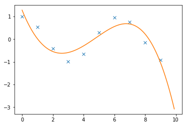
Interpolate between points:

x = np.arange(10)
y = np.cos(x)

Create interpolator

ay = interpolate.splrep(x,y,s=1)

Interpolate

xi = np.arange(0,10,0.1)
yi = interpolate.splev(xi,ay)

Plot:

import pylab as plt
plt.plot(x,y,'x',xi,yi)
plt.show()