pNbody tutorial
- official website : http://obswww.unige.ch/~revaz/pNbody/
- tutorial : http://obswww.unige.ch/~revaz/pNbody/rst/Tutorial.html
Using pNbody in the interpreter
First, load the python module:
In [1]:
from pNbody import *
Create an empty pNbody object and get info
In [2]:
nb = Nbody()
nb.info()
=================================================================================
TODO WARNING: A function that has not been fully written has been called.
TODO WARNING: This is most likely no reason to worry, but hopefully this message
TODO WARNING: will annoy the developers enough to start clean their code up.
TODO WARNING: Meanwhile, you can just carry on doing whatever you were up to.
=================================================================================
-----------------------------------
particle file       : ['file.dat']
ftype               : 'default'
mxntpe              : 6
nbody               : 0
nbody_tot           : 0
npart               : [0, 0, 0, 0, 0, 0]
npart_tot           : [0, 0, 0, 0, 0, 0]
mass_tot            : 0.0
byteorder           : 'little'
pio                 : 'no'
Create a pNbody object from positions:
In [4]:
pos = np.ones((10,3),np.float32)
nb = Nbody(pos=pos)
nb.info()
=================================================================================
TODO WARNING: A function that has not been fully written has been called.
TODO WARNING: This is most likely no reason to worry, but hopefully this message
TODO WARNING: will annoy the developers enough to start clean their code up.
TODO WARNING: Meanwhile, you can just carry on doing whatever you were up to.
=================================================================================
-----------------------------------
particle file       : ['file.dat']
ftype               : 'default'
mxntpe              : 6
nbody               : 10
nbody_tot           : 10
npart               : [10, 0, 0, 0, 0, 0]
npart_tot           : [10, 0, 0, 0, 0, 0]
mass_tot            : 1.0
byteorder           : 'little'
pio                 : 'no'

len pos             : 10
pos[0]              : array([1., 1., 1.], dtype=float32)
pos[-1]             : array([1., 1., 1.], dtype=float32)
len vel             : 10
vel[0]              : array([0., 0., 0.], dtype=float32)
vel[-1]             : array([0., 0., 0.], dtype=float32)
len mass            : 10
mass[0]             : 0.1
mass[-1]            : 0.1
len num             : 10
num[0]              : 0
num[-1]             : 9
len tpe             : 10
tpe[0]              : 0
tpe[-1]             : 0
Create a pNbody object using the ic module:
In [6]:
from pNbody import ic
nb = ic.plummer(10000,1,1,1,1,rmax=20.,M=1,name='plummer.dat',ftype='gadget')
comovingintegration = False
nb.write() # writes the nBody object to file 'plummer.dat' with the 'gadget' format (as specified in the Nbody object)
Read a pNbody from a file
In [8]:
nb = Nbody('plummer.dat',ftype='gadget')
The format is gadget
In [9]:
comovingintegration = False
In [10]:
nb.info()
-----------------------------------
particle file       : ['plummer.dat']
ftype               : 'gadget'
mxntpe              : 6
nbody               : 10000
nbody_tot           : 10000
npart               : [10000, 0, 0, 0, 0, 0]
npart_tot           : [10000, 0, 0, 0, 0, 0]
mass_tot            : 0.99999976
byteorder           : 'little'
pio                 : 'no'

len pos             : 10000
pos[0]              : array([ 0.08620726, -0.8825551 , -0.68550044], dtype=float32)
pos[-1]             : array([-0.6835583 ,  2.1199563 , -0.13416442], dtype=float32)
len vel             : 10000
vel[0]              : array([0., 0., 0.], dtype=float32)
vel[-1]             : array([0., 0., 0.], dtype=float32)
len mass            : 10000
mass[0]             : 1e-04
mass[-1]            : 1e-04
len num             : 10000
num[0]              : 0
num[-1]             : 9999
len tpe             : 10000
tpe[0]              : 0
tpe[-1]             : 0

atime               : 0.0
redshift            : 0.0
flag_sfr            : 0
flag_feedback       : 0
nall                : [10000, 0, 0, 0, 0, 0]
flag_cooling        : 0
num_files           : 1
boxsize             : 0.0
omega0              : 0.0
omegalambda         : 0.0
hubbleparam         : 0.0
flag_age            : 0
flag_metals         : 0
nallhw              : [0, 0, 0, 0, 0, 0]
flag_entr_ic        : 0
critical_energy_spec: 0.0
Get particle properties
Particle properties are numpy arrays of size nb.nbody:
In [11]:
nb.pos
Out[11]:
array([[ 0.08620726, -0.8825551 , -0.68550044],
       [-0.7158597 ,  1.8705164 , -0.16716339],
       [-0.0029057 , -0.03153811, -0.03678056],
       ...,
       [ 0.40189224,  0.11727811,  0.06398547],
       [-0.06060761, -0.17355472, -0.5085909 ],
       [-0.6835583 ,  2.1199563 , -0.13416442]], dtype=float32)
In [12]:
nb.vel
Out[12]:
array([[0., 0., 0.],
       [0., 0., 0.],
       [0., 0., 0.],
       ...,
       [0., 0., 0.],
       [0., 0., 0.],
       [0., 0., 0.]], dtype=float32)
In [13]:
nb.mass
Out[13]:
array([1.e-04, 1.e-04, 1.e-04, ..., 1.e-04, 1.e-04, 1.e-04], dtype=float32)
In [14]:
nb.num
Out[14]:
array([ 0, 1, 2, ..., 9997, 9998, 9999])
In [15]:
nb.tpe
Out[15]:
array([0, 0, 0, ..., 0, 0, 0])
Get the list of particle properties:
In [16]:
nb.get_list_of_array()
Out[16]:
['mass', 'num', 'pos', 'tpe', 'vel']
Display a model
# these two commands have been formatted differently so the website of the tutorial can be generated. # just copy them into a fresh interpreter cell and run them to see what they do. nb.show(size=(10,10)) nb.show(size=(20,20),shape=(256,256),palette='rainbow4')
In [17]:
Get physical values
positins x coordinates:
In [18]:
nb.x()
Out[18]:
array([ 0.08620726, -0.7158597 , -0.0029057 , ...,  0.40189224,
       -0.06060761, -0.6835583 ], dtype=float32)
center of mass
In [19]:
nb.cm()
Out[19]:
array([ 0.0013582 , -0.04152351, 0.01155748])
angular momentum:
In [20]:
nb.Ltot()
Out[20]:
array([0., 0., 0.], dtype=float32)
Compute potential and acceleration:
In [21]:
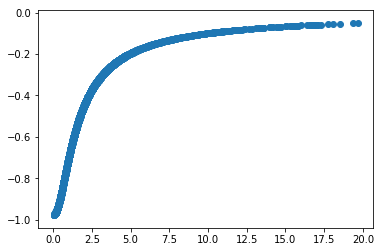
r   = nb.rxyz()
pot = nb.Pot(nb.pos,eps=0.1)
acc = nb.Accel(nb.pos,eps=0.1)
alternatively, you can use a treecode algorithm to compute the potential and acceleration (which is much faster):
In [22]:
pot = nb.TreePot(nb.pos,eps=0.1)
acc = nb.TreeAccel(nb.pos,eps=0.1)
create the tree : ErrTolTheta= 0.8
Plot:
In [24]:
import pylab as pt
pt.scatter(r, pot)
pt.show();    # for some reason the plot doesn't show up unless you put the semicolon here.
In [ ]: