Modeling a Gaussian Process over heterogeneous time series#
We consider here a physical process, such as stellar activity modulated by stellar rotation, affecting several observables (3 here) differently (different amplitudes, lags, etc.). We will model this physical process through a Gaussian process and its derivative. In this model, each observable is a linear combination of the GP (\(G(t)\)) and its derivative (\(G'(t)\)):
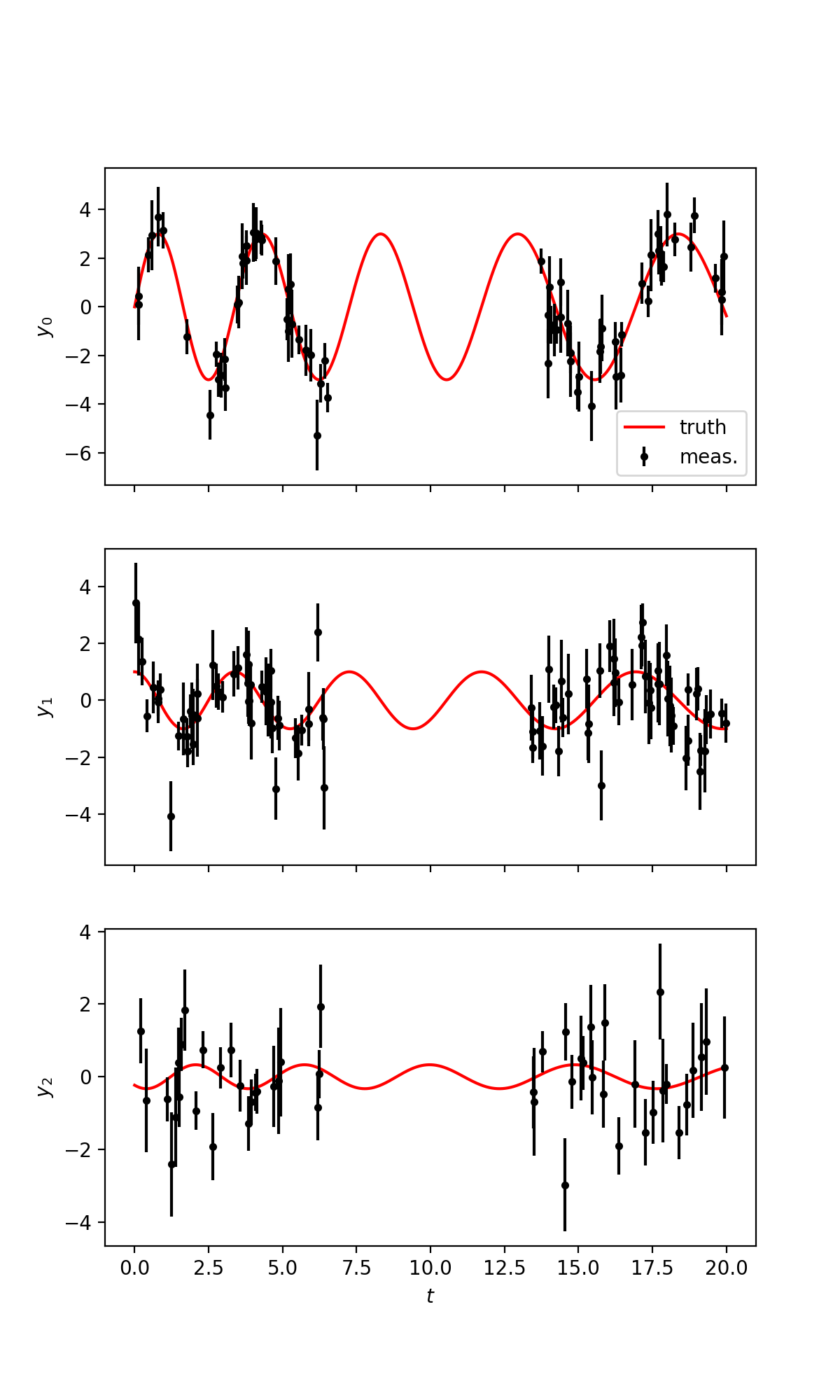
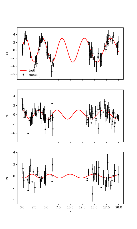
We first generate the 3 time series with a quasiperiodic evolution and different lags:
import numpy as np
import matplotlib.pyplot as plt

np.random.seed(0)

# Settings
P0 = 3.8
dP = 1.25
tmax = 20
amp = [3.0, 1.0, 0.33]
phase = [0, np.pi / 2, -3*np.pi / 4]
nt = [75, 100, 50]

# True signal
tsmooth = np.linspace(0, tmax, 2000)
Psmooth = P0 + dP * (tsmooth / tmax - 1 / 2)
Ysignal = [
  ak * np.sin(2 * np.pi * tsmooth / Psmooth + pk)
  for ak, pk in zip(amp, phase)
]

# Generate observations calendars
T = [
  np.sort(
  np.concatenate((np.random.uniform(0, tmax / 3,
  ntk // 2), np.random.uniform(2 * tmax / 3, tmax, (ntk + 1) // 2))))
  for ntk in nt
]

# Generate measurements with white noise
Yerr = [np.random.uniform(0.5, 1.5, ntk) for ntk in nt]
P = [P0 + dP * (tk / tmax - 1 / 2) for tk in T]
Y = [
  amp[k] * np.sin(2 * np.pi * T[k] / P[k] + phase[k]) +
  np.random.normal(0, Yerr[k]) for k in range(3)
]

# Plot
_, axs = plt.subplots(3, 1, sharex=True, figsize=(6, 10))
for k in range(3):
  ax = axs[k]
  ax.plot(tsmooth, Ysignal[k], 'r', label='truth')
  ax.errorbar(T[k], Y[k], Yerr[k], fmt='.', color='k', label='meas.')
  ax.set_ylabel(f'$y_{k}$')
ax.set_xlabel('$t$')
axs[0].legend()
(Source code, png, hires.png, pdf)
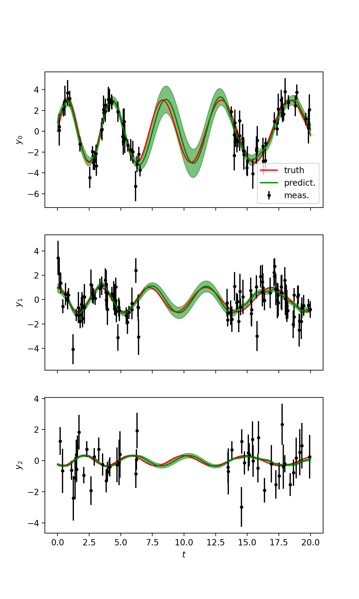
We now fit these data using S+LEAF:
from spleaf import cov, term
from scipy.optimize import fmin_l_bfgs_b

# Merge all 3 time series
t_full, y_full, yerr_full, series_index = cov.merge_series(T, Y, Yerr)

# Initialize the S+LEAF model
C = cov.Cov(t_full,
  err=term.Error(yerr_full),
  GP=term.MultiSeriesKernel(term.SHOKernel(1.0, 5.0, 1.0), series_index,
  np.ones(3), np.ones(3)))

# Fit the hyperparameters using the fmin_l_bfgs_b function from scipy.optimize.
# List of parameters to fit
param = C.param[1:]
# The amplitude of the SHOKernel is fixed at 1 (not fitted),
# since it would be degenerated with the amplitudes alpha, \beta.

# Define the function to minimize
def negloglike(x, y, C):
  C.set_param(x, param)
  nll = -C.loglike(y)
  # gradient
  nll_grad = -C.loglike_grad()[1][1:]
  return (nll, nll_grad)

# Fit
xbest, _, _ = fmin_l_bfgs_b(negloglike, C.get_param(param), args=(y_full, C))

# Use S+LEAF to predict the missing data
C.set_param(xbest, param)
_, axs = plt.subplots(3, 1, sharex=True, figsize=(6, 10))
for k in range(3):
  # Predict time series k
  C.kernel['GP'].set_conditional_coef(series_id=k)
  mu, var = C.conditional(y_full, tsmooth, calc_cov='diag')

  # Plot
  ax = axs[k]
  ax.plot(tsmooth, Ysignal[k], 'r', label='truth')
  ax.errorbar(T[k], Y[k], Yerr[k], fmt='.', color='k', label='meas.')
  ax.fill_between(tsmooth,
    mu - np.sqrt(var),
    mu + np.sqrt(var),
    color='g',
    alpha=0.5)
  ax.plot(tsmooth, mu, 'g', label='predict.')
  ax.set_ylabel(f'$y_{k}$')
ax.set_xlabel('$t$')
axs[0].legend()
plt.show()
(Source code, png, hires.png, pdf)
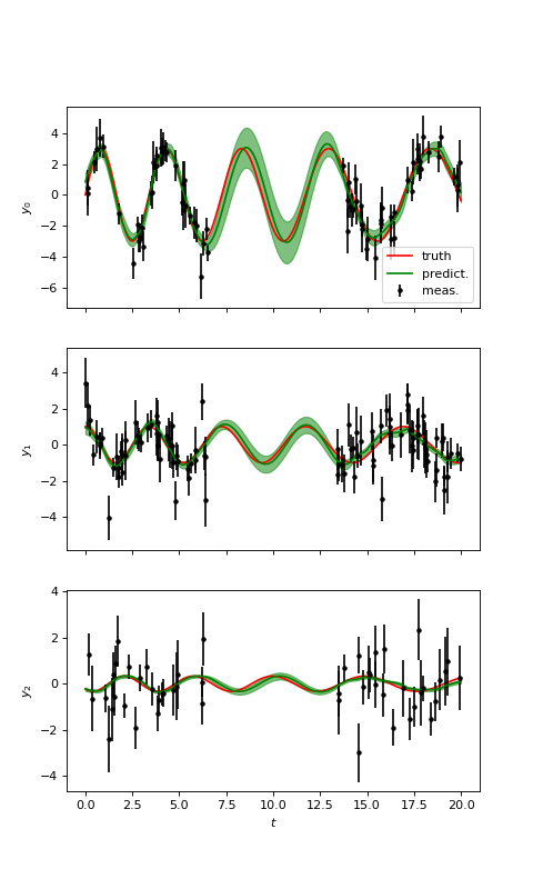
Thanks to the informations contained in the two first time series \(y_0\) and \(y_1\), we obtain a good prediction for the third time series \(y_2\), even if the signal to noise ratio is low.